Conclusion¶

I will refrain from stating conclusively that Dream boosted his Blaze rod drop and Ender pearl barter rate. To explain why, it is worth discussing stopping rules.

Stopping Rules¶

Both the MST and PE reports invoke stopping rules, though in a way that is not congruent with how they are used within the scientific community.

Suppose that a researcher is testing whether one variable influences another or is comparing two treatments or effect sizes. Suppose also that the researcher is primarily interested in whether there is an effect (or difference) and, if so, the direction of the effect. Finally, suppose that the researcher wants to set alpha at .05, which is to say, have a 5% probability of rejecting the null hypothesis of no effect, if it is true.

Using the fixed-sample stopping rule, the researcher would determine the number of subjects to be tested prior to performing the study. However, there is another type of stopping rule, called sequential stopping rules, which was first proposed by Wald in 1947. In a sequential stopping rule, the outcome ofthe statistical test could lead to testing more subjects. Thus, the number of subjects to be tested is not fixed in advance.[Fri98]

According to Wainer (2000) an adaptive test can be considered complete after a predetermined number of items have been administered, when a predetermined level of measurement precision has been reached, or when a predetermined length of time has elapsed. The two most commonly used methods for determining when a computerized adaptive test is complete are the fixed length and variable length stopping rules.

Under a fixed length stopping rule, an adaptive test is terminated when a predetermined number of items have been administered. Accordingly, all examinees are administered the same number of items, regardless of the degree of measurement precision achieved upon termination of the test. […]

In contrast, variable length stopping rules typically seek to achieve a certain degree of measurement precision for all examinees, even when doing so means that some examinees are given more items than others. Two types of variable length stopping rules have been used (Dodd, Koch, & De Ayala, 1993). These are the standard error (SE) stopping rule and the minimum information stopping rule. Of these, the most commonly used has been the SE stopping rule, which terminates an adaptive test when a predetermined standard error has been reached for the most recent examinee trait estimate (Boyd, Dodd, & Choi, 2010).[CGD10]

One criticism of rules like O’Brien and Fleming is their rigidity in requiring a fixed maximum number of preplanned interim analyses. Greater flexibility is possible with the Peto-Haybittle rule, which simply specifies a fixed p value (often \(p<0.001\)) for stopping early. For example, the European myocardial infarction amiodarone trial (EMIAT) is an ongoing study of 1500 patients at high risk after myocardial infarction comparing amiodarone (an antiarrhythmic drug) with placebo. Two year mortality is the primary end point, and the stopping guideline for efficacy is \(p < 0.001\) in favour of amiodarone.[Poc92]

A clear stopping rule is necessary when the number of datapoints you could look at is practically infinite; we could survey every single person in the United States to determine their political views, but it is more feasible to pick a large enough sample of them to achieve a certain statistical accuracy. Alternatively, we could flip between data gathering and analysis until our target accuracy or statistical measure is reached, but this risks coming to a premature stop due to statistical fluctuations; had we just analyzed X more datapoints, our test statistic would switch from “statistically significant” to “not statistically significant” and our declaration of significance would be premature.

Dream has not completed a practically infinite number of random-seed any-percent Minecraft 1.16 runs, however. If our hypothesis is that Dream boosted his drop/barter rate since returning to that speedrun category, then the entire dataset consists of thirty-three runs where Blazes were killed for Blaze rods, and twenty-two runs where Ender pearls were bartered for, spread across six streaming sessions. There is no more data to be collected, and the data that is present is nowhere near large enough to pose an analytic challenge. If those datapoints were insufficient to establish the hypothesis, then a well-designed statistical test metric will conclude the evidence is inconclusive. If the fluctuations could be due to chance, then a well-designed metric will take that into account. The data cannot be cherry-picked to artificially boost the metric, as the MST report examines every applicable cherry.

The imposition of a binary decision threshold on continuous test statistics, and the resulting necessity of stopping rules, has led some researchers to call for the abandonment of statistical significance entirely.[MGG+19] Rather than have the researcher or publisher check if p-values or Bayes factors cross a certain threshold, they propose researchers and publishers take a holistic approach that also factors in “related prior evidence, plausibility of mechanism, study design and data quality, real world costs and benefits,” and “novelty of finding” among other things.

As an outsider to the Minecraft speedrunning community, I do not have full knowledge of prior evidence. I do not have a good understanding of the costs or benefits of removing Dream’s speed-running records, and should I make the wrong decision I will not pay the consequences. The best thing I can do is to instead lay out my full reasoning as clearly I can. If the community accepts the premises behind my arguements and can find few flaws in how I link them together, they are in a much better position to translate a continuous Bayes factor into a binary decision.

Lindley’s Paradox¶

This analysis might seem like a waste: both the MST and PE reports conclude Dream cheated, and this report only avoids saying so because it is not the author’s place to. If frequentist and Bayesian methods always come to the same conclusion, why does it matter which we choose?

Let’s do a case study of Benex, another speedrunner the MST report gathered data on. Rather than repeat the prior chart, we’ll add a simple frequentist analysis of Benex’s data that uses a cumulative p-value.

# Execute this cell to install all dependencies. Apologies for the spam.

# If you're running this on your own computer, I recommend altering "install mpmath" 
#  to read "install --user mpmath", that way you don't need administrator access.
# On Colab, change "pip -q install" to "pip install", as otherwise you could miss a message
#  that you need to restart your runtime. If you don't restart, the code won't work.
# A few error messages are fine, I usually get one about mismatched versions and the code
#  still runs. 

!pip -q install mpmath myst_nb numpy pandas matplotlib scipy

from fractions import Fraction

from math import log,factorial
import matplotlib.pyplot as plt
from mpmath import mp
from myst_nb import glue

import numpy as np

import pandas as pd
from scipy.optimize import differential_evolution
from scipy.stats import beta,binom,nbinom


dpi         = 200  # change this to increase/decrease the resolution charts are made at
book_output = True ### changing this to False will allow you to view the plots in a Jupyter notebook

def fig_show( fig, name ):
    """A helper to control how we're displaying figures."""
    global book_output
    
    if book_output:
        glue( name, fig, display=False )
        plt.close();
    else:
        fig.show()

# missing "simple_bernoulli_bf.py"? Uncomment this line to grab it from the repository
# !wget -c "https://raw.githubusercontent.com/hjhornbeck/bayes_speedrun_cheating/main/simple_bernoulli_bf.py"

from simple_bernoulli_bf import prior, posterior_H_fair, BF_H_fair_H_cheat

# missing the data files? Uncommenting and running this cell might retrieve them

# !mkdir data
# !wget -cP data "https://raw.githubusercontent.com/hjhornbeck/bayes_speedrun_cheating/main/data/blaze.benex.tsv"
# !wget -cP data "https://raw.githubusercontent.com/hjhornbeck/bayes_speedrun_cheating/main/data/bartering.benex.tsv"

colours = ['b', 'g', 'r', 'c', 'm', 'y', 'k']  # makes colouring some of the following easier
colours = colours + colours                    # double-up to allow for extra data

blaze_players = ['benex']
pearl_players = blaze_players

blaze_rods = {p:pd.read_csv(f'data/blaze.{p}.tsv',sep="\t") for p in blaze_players}
bartering  = {p:pd.read_csv(f'data/bartering.{p}.tsv',sep="\t") for p in pearl_players}

blaze_rods['benex'].set_index('n').transpose()

n	11	15	14	8	13	12	16	14	7	14	11
k	6	7	6	7	6	7	7	10	3	5	8

fig, (ax1,ax2) = plt.subplots(nrows=1, ncols=2, figsize=(8, 4), dpi=dpi, facecolor='w', edgecolor='k')

i = 0       # allow for copy-paste code
p = 'benex'


# Blaze rods first
r_fair = Fraction(1,2)
priors = [prior( r_fair, scale ) for scale in [Fraction(4,3), 4, 12]]

count = len(blaze_rods[p])
x     = np.arange(1, count+1)
sum_n = np.cumsum( blaze_rods[p]['n'] )
sum_k = np.cumsum( blaze_rods[p]['k'] )

# p-values 
y = [1 - binom.cdf( sum_k[i], sum_n[i], float(r_fair) ) for i in range(count)]
ax1.plot( x, y, '-r', label="blaze rods" )

# my Bayes factor
y = [BF_H_fair_H_cheat(sum_k[i], sum_n[i], r_fair, *priors[1]) for i in range(count)]
ax2.plot( x, y, '-r' )
    
y_low = [BF_H_fair_H_cheat(sum_k[i], sum_n[i], r_fair, *priors[0]) for i in range(count)]
y_hig = [BF_H_fair_H_cheat(sum_k[i], sum_n[i], r_fair, *priors[2]) for i in range(count)]
ax2.fill_between( x, [float(v) for v in y_low], [float(v) for v in y_hig], \
                     alpha=0.2, color='r' )


# Ender pearls
r_fair = Fraction(20, 423)
priors = [prior( r_fair, scale ) for scale in [Fraction(4,3), 4, 12]]

count = len(bartering[p])
x     = np.arange(1, count+1)
sum_n = np.cumsum( bartering[p]['n'] )
sum_k = np.cumsum( bartering[p]['k'] )

# p-values
y = [1 - binom.cdf( sum_k[i], sum_n[i], float(r_fair) ) for i in range(count)]
ax1.plot( x, y, '-b' )
glue( 'benex_pval_12', y[11], display=False )

# my Bayes factor
y = [BF_H_fair_H_cheat(sum_k[i], sum_n[i], r_fair, *priors[1]) for i in range(count)]
ax2.plot( x, y, '-b', label="pearl barters" )
glue( 'benex_bf_12', float(y[11]), display=False )

y_low = [BF_H_fair_H_cheat(sum_k[i], sum_n[i], r_fair, *priors[0]) for i in range(count)]
y_hig = [BF_H_fair_H_cheat(sum_k[i], sum_n[i], r_fair, *priors[2]) for i in range(count)]
ax2.fill_between( x, [float(v) for v in y_low], [float(v) for v in y_hig], \
                     alpha=0.2, color='b' )


# add the trimmings to both charts
x = range( 1, max(len(blaze_rods[p]), len(bartering[p])) )
ax1.plot( x, [0.05 for v in x], '--k', label='p = 0.05' )
ax1.plot( x, [0.001 for v in x], '--k', label='p = 0.001' )

ax2.plot( x, [19 for v in x], '--k', label='19:1' )
ax2.plot( x, [1 for v in x], '--k', label='break even' )

          
ax1.set_xlabel("run")
ax1.set_xticks([1,len(blaze_rods['benex']),len(bartering['benex'])])
ax1.set_ylabel('p-value')
ax1.set_yscale("log")

ax2.set_xlabel("run")
ax2.set_xticks([1,len(blaze_rods['benex']),len(bartering['benex'])])
ax2.set_ylabel('H_fair / H_cheat')
ax2.set_yscale("log")

ax1.legend()
ax2.legend()
          
fig_show( fig, 'fig:benex_both' )

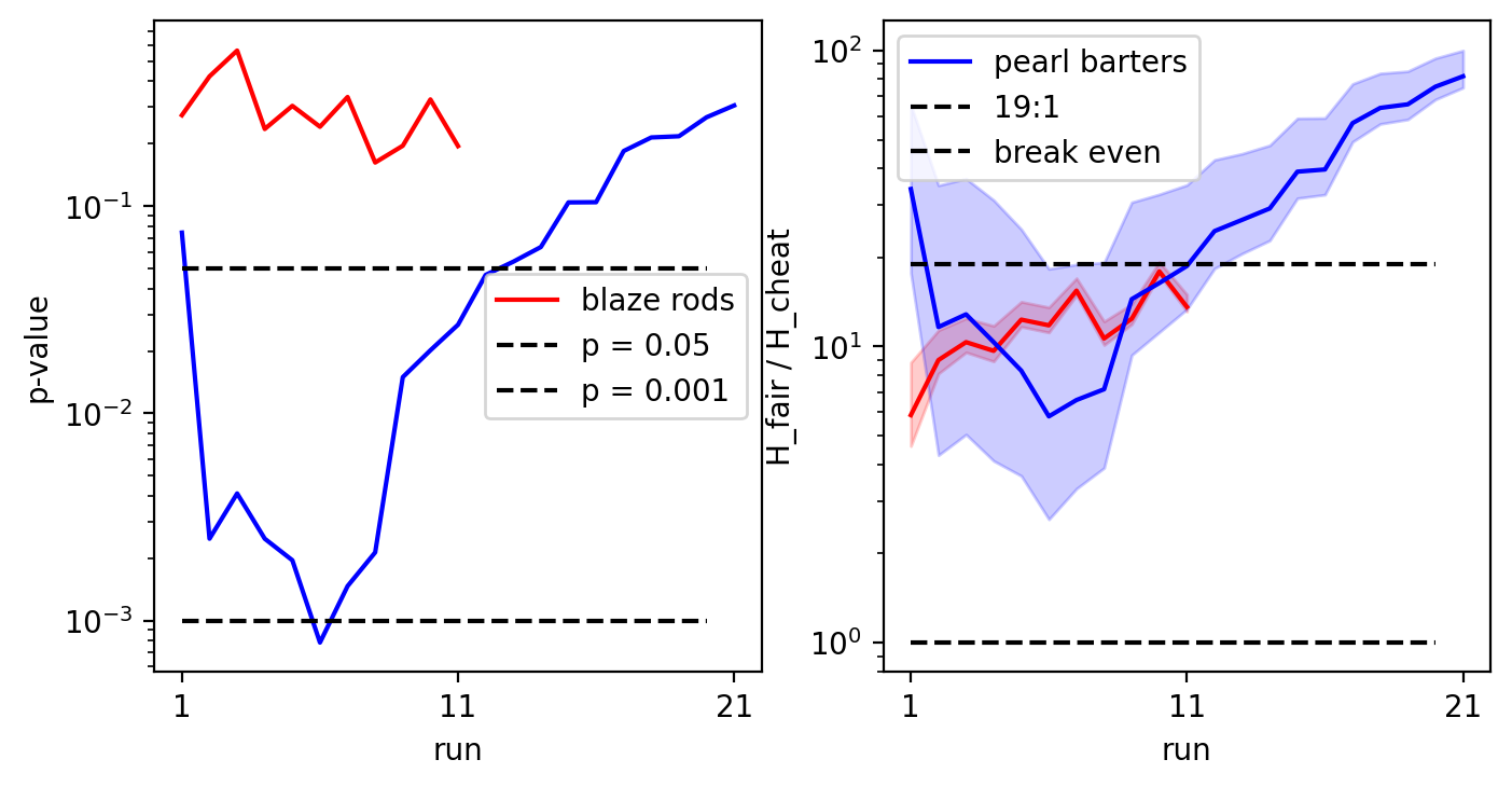
Fig. 20 A comparison of p-values and my Bayes factor for Benex’s record on Blaze rod drops and Ender pearl barters. Both metrics are calculated according to the cumulative \(n\) and \(k\) as of that run.¶

I should point out that this imagined world is not our own. The MST team applied corrections for multiple comparisons that would likely have watered down the p-value. Benex’s first five runs were part of one stream, while his next three were in a second stream, so the run that crossed the line was at the start of a new stream and followed by two runs that watered down his p-values. It’s highly unlikely Benex switched their Ender pearl barter rate mid-stream, so that sixth run can be safely discarded as an outlier.

These graphs tell two very different stories. We could imagine a universe where the Minecraft Speedrunning Team invoked the Peto-Haybittle stopping rule, as it is well-regarded though considered too conservative for some researchers.[SG05] When Benex’s p-value crossed the \(p < 0.001\) threshold on his sixth run, they declared him to have cheated and striped him of any records he held.

We could also imagine a universe where the MST invoked my Bayes prior, observed the exact same streams, noted Benex’s odds of fair play never dipped below 6:1 for my choice of prior, and did nothing. At no point would this universe’s MST believe Benex tweaked his Ender pearl barter rate.

This is a weak example of Lindley’s Paradox.

An example is produced to show that, if H is a simple hypothesis and x the result of an experiment, the following two phenomena can occur simultaneously:
(i) a significance test for H reveals that x is significant at, say, the 5% level;
(ii) the posterior probability of H, given x, is, for quite small prior probabilities of H, as high as 95%.
Clearly the common-sense interpretations of (i) and (ii) are in direct conflict. The phenomenon is fairly general with significance tests and casts doubts on the meaning of a significance level in some circumstanices.[Lin57]

On the twelfth run, Benex’s cumulative p-value is 0.047, while my Bayes factor is about 24.5:1, which crosses the 95% line when translated to a percentage. Dream’s data may be strong enough to point in one direction, but the data from other speedrunners may not. Indeed, anyone interested in cheating would likely decrease their advantage below what was listed in the PE report or this one, increasing the odds of achieving Lindley’s paradox.

The debate between frequentist and Bayesian statistics can have a real-world consequences, and is not to be dismissed lightly.

Did Dream Cheat? A Bayesian Analysis of a Bernoulli Process.

Conclusion¶

Stopping Rules¶

Lindley’s Paradox¶