Simulation Results
As nice as all that mathematics was, it means nothing if this Bayes factor doesn’t work as advertised. If it doesn’t increase when a person plays with an unaltered copy of the game, and if it doesn’t decrease when a cheater modifies their drop or barter rate, then it is useless no matter what the math tells us.
Modifying a copy of Minecraft 1.16.1 and doing speed runs is a time-consuming process, but we have a viable alternative: since the decision of whether to drop a Blaze rod or collection of Ender pearls is a Bernoulli process, it can be perfectly simulated by any other Bernoulli process. Pseudo-random number generators are a particularly good choice for this, as the probability of success can be controlled directly. We must still take care to match the behaviour of Minecraft speedrunners as closely as we can, of course.
# Execute this cell to install all dependencies. Apologies for the spam.

# If you're running this on your own computer, I recommend altering "install mpmath"
#  to read "install --user mpmath", that way you don't need administrator access.
# On Colab, change "pip -q install" to "pip install", as otherwise you could miss a message
#  that you need to restart your runtime. If you don't restart, the code won't work.
# A few error messages are fine, I usually get one about mismatched versions and the code
#  still runs.

!pip -q install mpmath myst_nb numpy pandas matplotlib scipy
from fractions import Fraction

from math import log,factorial
import matplotlib.pyplot as plt
from mpmath import mp
from myst_nb import glue

import numpy as np

import pandas as pd
from scipy.optimize import differential_evolution
from scipy.stats import beta,binom,nbinom


dpi         = 200  # change this to increase/decrease the resolution charts are made at
book_output = True # changing this to False will make it easier to view plots in a Jupyter notebook

def fig_show( fig, name ):
    """A helper to control how we're displaying figures."""
    global book_output

    if book_output:
        glue( name, fig, display=False )
        plt.close();
    else:
        fig.show()
# missing "simple_bernoulli_bf.py"? Uncomment this line to grab it from the repository
# !wget -c "https://raw.githubusercontent.com/hjhornbeck/bayes_speedrun_cheating/main/simple_bernoulli_bf.py"

from simple_bernoulli_bf import prior, posterior_H_fair, BF_H_fair_H_cheat
Blaze Rod Drops
Blaze rod drops are the easiest to model, as it almost certainly follows the Negative Binomial distribution. To try and match what actual speedrunners do, we’ll load up all the data from the MST report and pool it together.
# missing the data files? Uncommenting and running this cell might retrieve them

# !mkdir data
# !wget -cP data "https://raw.githubusercontent.com/hjhornbeck/bayes_speedrun_cheating/main/data/blaze.benex.tsv"
# !wget -cP data "https://raw.githubusercontent.com/hjhornbeck/bayes_speedrun_cheating/main/data/blaze.dream.tsv"
# !wget -cP data "https://raw.githubusercontent.com/hjhornbeck/bayes_speedrun_cheating/main/data/blaze.illumina.tsv"
# !wget -cP data "https://raw.githubusercontent.com/hjhornbeck/bayes_speedrun_cheating/main/data/blaze.sizzler.tsv"
# !wget -cP data "https://raw.githubusercontent.com/hjhornbeck/bayes_speedrun_cheating/main/data/blaze.vadikus007.tsv"
# create a blank dataframe to store all this data in
all_blaze_rods = pd.DataFrame( {'n':[], 'k':[]} )


# the Ender pearl stats have slightly different names
blaze_players = ['benex','dream','illumina','sizzler','vadikus007']

# load in the data
for p in blaze_players:
    all_blaze_rods = all_blaze_rods.append( pd.read_csv(f'data/blaze.{p}.tsv',sep="\t") )


fig = plt.figure(figsize=(8, 4), dpi=dpi, facecolor='w', edgecolor='k')


# pull out all the unique values to be the X axis along our bar chart
blaze_k = sorted( all_blaze_rods['k'].unique() )
plt.bar( blaze_k, [all_blaze_rods['k'][ all_blaze_rods['k'] == k ].count() for k in blaze_k], \
        label='blaze rods gathered' )

plt.xlabel('blaze rods gathered')
plt.ylabel('number of runs where k rods were gathered')
plt.yticks([0,15,30])

fig_show( fig, 'fig:blaze_rods_gathered' )
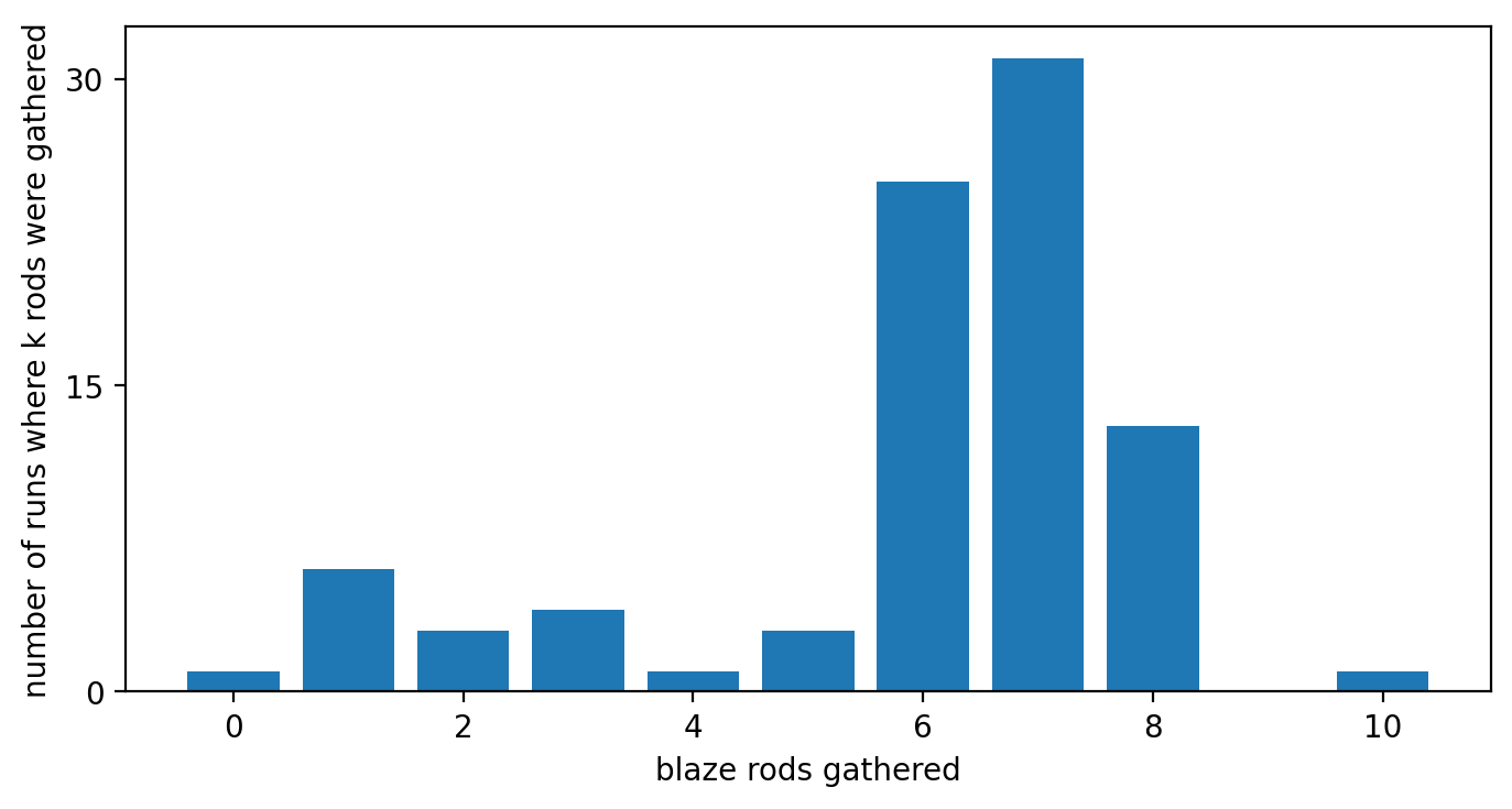
Fig. 10 The number of Blaze rods gathered during runs from five separate top-level speedrunners, according to the Minecraft Speeedrunning Team.
The Mechanics of Blaze Rods
There’s a surprising amount of variance in the number of Blaze rods gathered, given the game mechanics involved.
Accessing The End requires finding a Stronghold, and finding that requires tossing Eyes of Ender to point out the direction of the Stronghold. Triangulating the location requires a minimum of two Eyes, and there’s a one in five chance an Eye will break when tossed. Once found, players must find a portal within the Stronghold that grants them access to The End. This portal is powered by twelve Eyes of Ender, which have a one-in-ten chance of spontaneously appearing in an appropriate spot. Do the math, and the most common outcome is to have one Eye of Ender already in the portal, while three or more Eyes are present 34.1% of the time.
Eyes of Ender are crafted by combining Ender pearls with Blaze powder. Two items of the latter can be created from one Blaze rod. Given all of the above, the safest route is to kill Blazes until the runner has seven Blaze rods, which allows for fourteen Blaze powders and thus fourteen Eyes of Ender. Even if two Eyes of Ender break when finding the Stronghold, which has a 4% chance of happening, the runner has enough Eyes to fill an empty portal.
While the safest route is indeed the most common one, a substantial number of speedruns collected only six rods. This is a viable route, as immediate entry to The End either requires no Eyes break while finding the stronghold (64% odds), only one Eye breaks but the portal has at least one Eye already present (about 23% odds), or both eyes break but two or more Eyes are present (about 1.4%). Surprisingly, a number of runners also collected eight rods. This may be because the runner wasn’t confident they could find the Stronghold with just two Eyes and wanted some safety margin.
Five rods is the bare minimum I could see used to complete a speed run, as the odds of a runner with only eight Eyes of Ender keeping both the ones they toss and finding four or more in the End portal are only 1.6%. The low-rod runs were likely aborted due to other reasons. That one run of ten rods comes from Benex, and the comments about going after Wither skeletons suggest it wasn’t a typical speedrun.
In real life, speed runners pick a range of Blaze rod targets, so our simulation should do the same. We’ll discard all the recorded runs where less than five and more than eight rods were collected, and use their relative frequencies to pick 200 values for \(k\). We’ll then create three universes: one where players with an unmodified game have \(\vec k\) for Blaze rod targets, one where players boost their drop odds for the same targets, and one where players reduce their odds. Since one random simulation doesn’t give you a feel for the variation present, we’ll run 16 distinct players for each of the three scenarios just mentioned.
random  = np.random.default_rng(42)

# generate the weights and normalize
weights = np.array( [all_blaze_rods['k'][ all_blaze_rods['k'] == k ].count() for k in range(5,9)] )
weights = weights / np.sum(weights)

r_fair    = 0.5
r_cheat_h = 0.569 ; glue( 'sim_blaze_r_cheat_h', r_cheat_h*100, display=False )
r_cheat_l = 0.431 ; glue( 'sim_blaze_r_cheat_l', r_cheat_l*100, display=False )
count     = 200   ; glue( 'sim_blaze_count', count, display=False )
clones    = 16    ; glue( 'sim_blaze_clones', clones, display=False )
a_prior, b_prior   = prior(r_fair, 4)

x      = np.arange(1, count+1)
k      = 5 + random.choice( 4, size=(clones,count), p=weights )
sum_k  = np.cumsum( k, axis=1 )

cheat_h_nk = random.negative_binomial( k, r_cheat_h )
cheat_l_nk = random.negative_binomial( k, r_cheat_l )
fair_nk    = random.negative_binomial( k, r_fair )

sum_k         = np.cumsum( k, axis=1 )
sum_cheat_h_n = sum_k + np.cumsum( cheat_h_nk, axis=1 )
sum_cheat_l_n = sum_k + np.cumsum( cheat_l_nk, axis=1 )
sum_fair_n    = sum_k + np.cumsum( fair_nk, axis=1 )


fig = plt.figure(figsize=(8, 4), dpi=dpi, facecolor='w', edgecolor='k')

for idx in range(clones):
    y = [BF_H_fair_H_cheat(sum_k[idx][i], sum_cheat_h_n[idx][i], r_fair, a_prior, b_prior) for i in range(count)]
    if idx == 0:
        plt.plot( x, y, '-r', label=f'cheater (r={r_cheat_h:.3f})' )
    else:
        plt.plot( x, y, '-r', alpha=0.1 )

    y = [BF_H_fair_H_cheat(sum_k[idx][i], sum_cheat_l_n[idx][i], r_fair, a_prior, b_prior) for i in range(count)]
    if idx == 0:
        plt.plot( x, y, '-b', label=f'cheater (r={r_cheat_l:.3f})' )
    else:
        plt.plot( x, y, '-b', alpha=0.1 )

    y = [BF_H_fair_H_cheat(sum_k[idx][i], sum_fair_n[idx][i], r_fair, a_prior, b_prior) for i in range(count)]
    if idx == 0:
        plt.plot( x, y, '-k', label=f'fair (r={r_fair:.3f})' )
    else:
        plt.plot( x, y, '-k', alpha=0.1 )

plt.plot( x, [1 for v in x], '--g', label='break even' )

plt.xlabel("rounds")
plt.xticks([1,count])
plt.ylabel('H_fair / H_cheat')
plt.yscale("log")

plt.legend()
fig_show( fig, 'fig:sim_blaze_trio' )
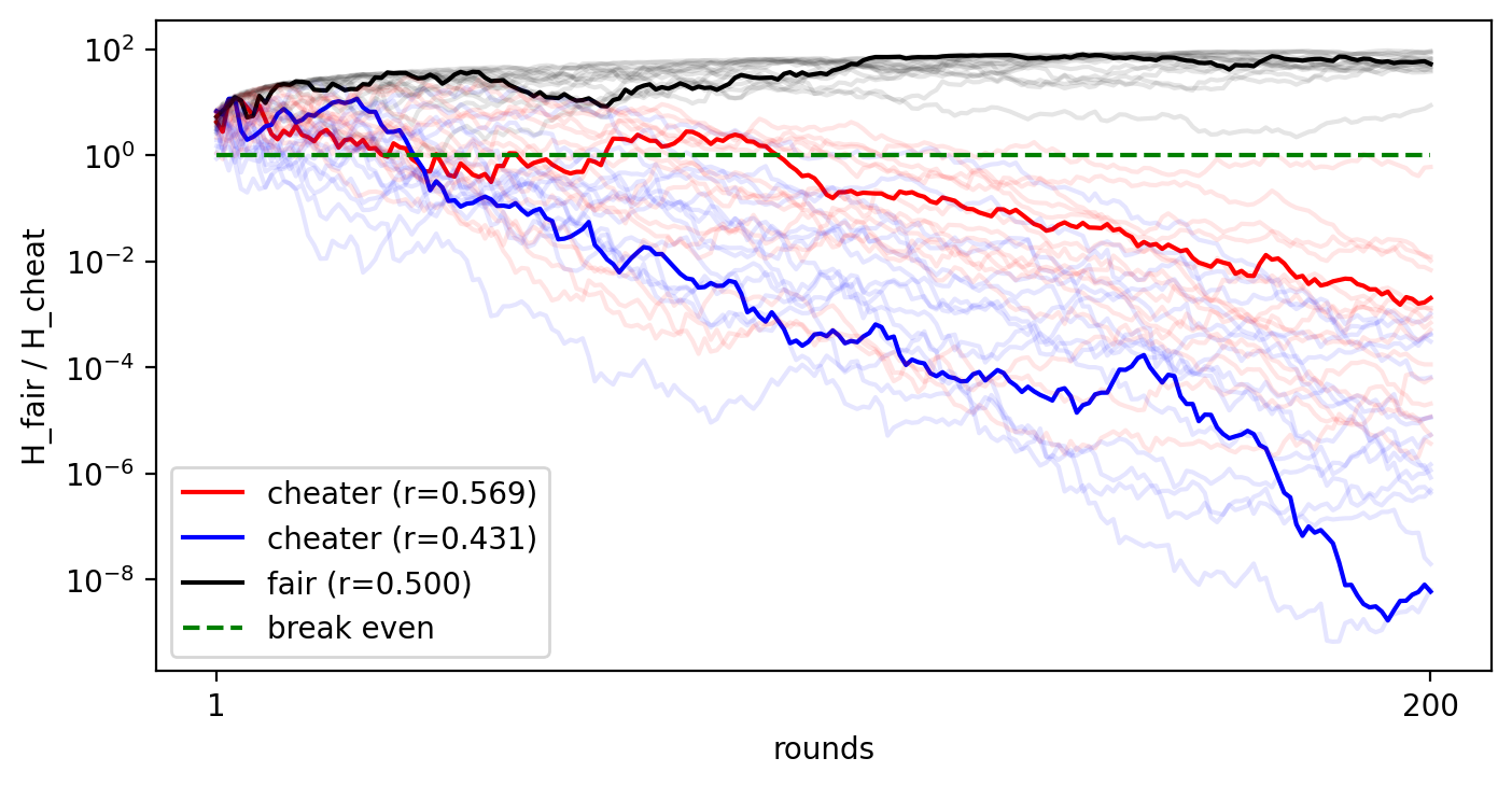
Fig. 11 The behaviour of this Bayes Factor for 16 clones of three players that had different Blaze rod drop rates. One group of 16 clones had the usual drop rate, one group increased it to 56.9%, and one decreased it to 43.1%.
There are two distinct behaviours. For players with unmodified drop rates, the Bayes factor usually stays above one and appears to shadow the \(\sqrt{n}\) trajectory detailed earlier. For the two cheating players, the Bayes factor gradually drifts below one and in some cases gets below 1:1,000,000 odds of playing fair. There’s a bit of variation, though, as one of the fair players’ Bayes factors drifts downward toward the 1:1 odds range, and one of the cheaters manages roughly 1:1 odds of fair play during the entire session. There are also times where the cheating players have Bayes factors that suggest fair play, those these usually only happen during the first rounds.
Interestingly, the cheater that reduced their odds of a Blaze rod drop seems to have fared worse than the player that boosted their Blaze rod drops. One explanation is that while the Negative Binomial may be treated the same as the Binomial in the long run, always stopping on a positive will skew the results in the short term.
Cheating Techniques
Why would a cheater want to reduce the number of Blaze rods they collect? Put yourself behind their keyboard. They know that the odds of being detected are high if they simply increase their drop rate. Someone watching the stream will get suspicious, count up Blaze rods, and alert others.
A big-brained alternative is to temporarily elevate the drop rate. We’re used to thinking of people getting lucky from time to time, so a short run of unusually good luck might pass under the radar. Even if it doesn’t, the cheater has a plausible excuse. They can train during the sessions with the fair drop rate, and only start cheating when they’re skilled enough to earn a record.
One problem: for them, it will always be true that \(\|\vec k\|_1 > r_\text{fair}\|\vec n\|_1\). No one may be able to detect their cheating in the short term, but a career-long analysis will show an elevated success rate relative to non-cheating players. The more times this cheater temporarily boosts their luck, the greater the evidence they’ve done exactly that.
A galaxy-brained move is to alternate between short periods of elevated drop rates and long periods of deflated drop rates. The PE report considers multiple “boost rates” for Ender pearl barters, but never considers deflated rates. The MST report states that apparently elevated drop rates made the speedrunning community suspicious of Dream (pg. 3), and that any runner “observed experiencing such unlikely events would be held to the same level of scrutiny” (pg. 4); the flip side is that any runner experiencing an unusually low number of drops would not. This blind spot of the speedrunning community could be exploited: by altering their drop rate both up and down, a cheating speedrunner can ensure their career stats do not reveal evidence of cheating.
Greatly reducing their drop rate creates a large handicap to overcome, even if it does mean they can punch the “cheat” button pretty often. Instead, long periods of slightly-decreased luck would reduce the handicap and allow the cheater to exploit unusually good luck during their grind times. Should one of their elevated periods raise suspicion, not only can they pull out the “I got lucky” excuse, they can also point to a specific period of prior attempts and argue that, when taken as a whole, all the evidence demonstrates their drop rate is normal. The PE report analyzed the six attempts the MST report did for evidence of elevated drop rates, as well as those six plus five attempts Dream catalogued, but never considered analyzing those five attempts in isolation.
To be clear, I’m not accusing Dream of either type of cheating. I’ve deliberately avoided doing the appropriate analysis before writing this text, in fact. When analyzing both reports for flaws, though, this oversight is easy to spot. It is also easy to detect, once you know what to look for, and the Bayes factor I’ve created is sensitive to both increased and decreased drop rates. An analysis that uses p-values might also be able to detect this if a “two-tailed” p-value is used, but the MST report opted to use a “one-tailed” p-value instead.
Ender Pearl Barters
This analysis has focused on Blaze rods drops because they are so easy to understand. They can be directly analogized to the flip of a coin, and quite clearly follow a Negative Binomial, so the choice of simulation is very clear. None of the above math assumed a fifty-fifty success rate, nor whether the numbers were better modelled by the Negative Binomial or Binomial distributions. It should work flawlessly with Ender pearl barters.
Our simulation, on the other hand, must choose between the Negative Binomial or Binomial.
# missing the data files? Uncommenting and running this cell might retrieve them

# !wget -cP data "https://raw.githubusercontent.com/hjhornbeck/bayes_speedrun_cheating/main/data/bartering.benex.tsv"
# !wget -cP data "https://raw.githubusercontent.com/hjhornbeck/bayes_speedrun_cheating/main/data/bartering.dream_before.tsv"
# !wget -cP data "https://raw.githubusercontent.com/hjhornbeck/bayes_speedrun_cheating/main/data/bartering.dream_after.tsv"
# !wget -cP data "https://raw.githubusercontent.com/hjhornbeck/bayes_speedrun_cheating/main/data/bartering.illumina.tsv"
# !wget -cP data "https://raw.githubusercontent.com/hjhornbeck/bayes_speedrun_cheating/main/data/bartering.sizzler.tsv"
# !wget -cP data "https://raw.githubusercontent.com/hjhornbeck/bayes_speedrun_cheating/main/data/bartering.vadikus007.tsv"
# create a blank dataframe to ensure the proper format
all_pearl_barters = pd.DataFrame( {'n':[], 'k':[]} )


# the Blaze rod stats have slightly different names
pearl_players = ['benex','dream_before','dream_after','illumina','sizzler','vadikus007']

# load in the data
for p in pearl_players:
    all_pearl_barters = all_pearl_barters.append( pd.read_csv(f'data/bartering.{p}.tsv',sep="\t") )


fig = plt.figure(figsize=(8, 4), dpi=dpi, facecolor='w', edgecolor='k')

# pull out all the unique values for the X axis
pearl_k = sorted( all_pearl_barters['k'].unique() )
plt.bar( pearl_k, [all_pearl_barters['k'][ all_pearl_barters['k'] == k ].count() for k in pearl_k], \
        label='ender pearl barters' )

plt.xlabel('successful barters')
plt.ylabel('number of runs where k barters were successful')
plt.yticks([0,25,50])

fig_show( fig, 'fig:ender_pearl_barter' )
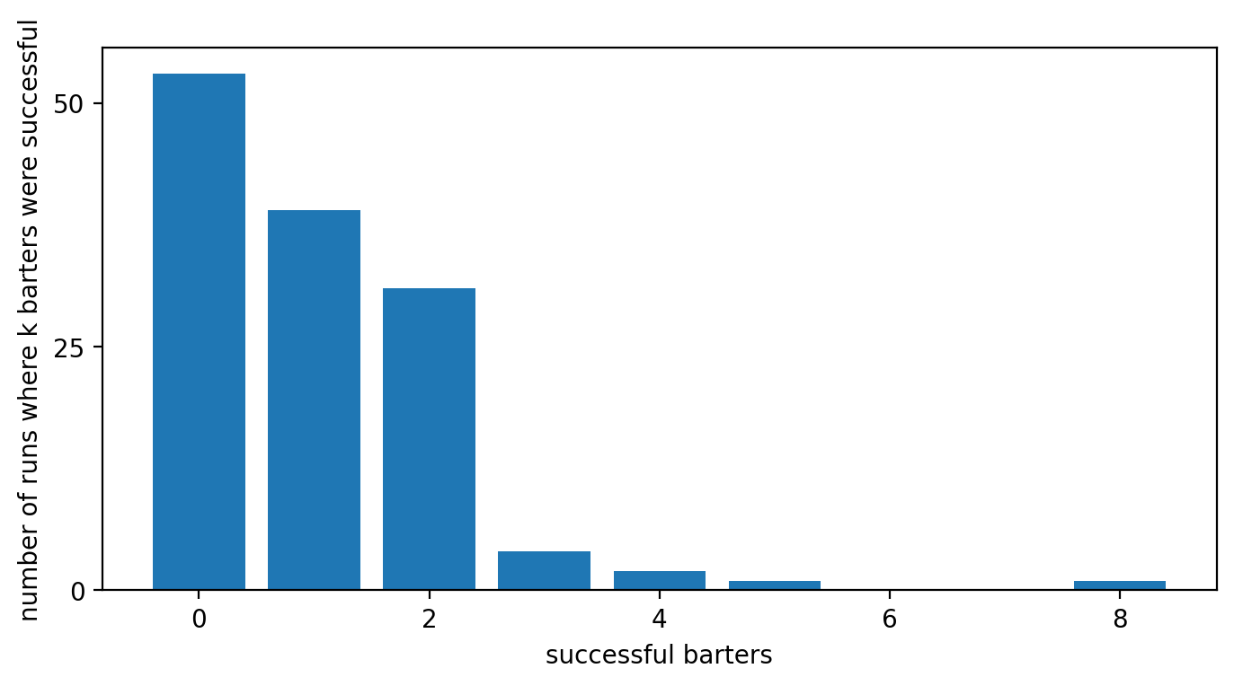
Fig. 12 The number of Ender pearl barters performed during a speedrun, according to the Minecraft Speeedrunning Team.
In Overuse of the Negative Binomial, I gave a theoretical argument for why Ender pearl barters may not follow a Negative Binomial distribution. Now we have an empirical argument. Bartering with Piglins is supposed to be the primary way to earn Ender pearls in a random-seed any-percent Minecraft 1.16 speedrun, and yet most speed runners earned zero Ender pearls via this method?
The easiest explanation is that few of the runs in the MST report were successful. Players usually target a specific number of Ender pearls, but barters drop anywhere from four to eight pearls. Assuming uniform odds, two Ender pearl barters have a 60% chance of giving twelve or more pearls, and as long as none of the resulting Eyes of Ender break while finding the Stronghold the runner can immediately go to The End. Half the time, it takes anywhere from two to thirty-five barters for a speed runner to earn two Ender pearl barters. Conversely, this means that half the time a player will have to wait longer than three and a half minutes to earn those barters, a serious problem if you are on the clock. If we assume that Minecraft 1.16 runners always target two barters, then only a quarter of all speed runs are successful. If players only stop bartering if they are out of time or earn those two barters, then that success rate implies they budget for twenty barters, which requires exactly two minutes to complete, and abort if they fail to hit that target.
Of course, that assumes quite a bit. Endermen have a fifty-fifty chance of dropping an Ender pearl when killed. While they rarely spawn in most Minecraft biomes, one notable exception is Nether Warped forest. A player that happens to stumble on such a biome can use that instead to gather Ender pearls. Barters also require gold ingots, so it is also possible for a speed runner to abort if they run out of gold instead of time. Theoretically, it’s also possible to get to The End with just one Ender pearl barter. There’s a 20% chance of getting eight Ender pearls at once and a 50% chance of picking up two more via killing two to three Enderman, which gives the runner a 25% chance of jumping immediately to The End once they’ve found the Stronghold. The overall odds of that happening are about 2.5%, but a speedrunner may prefer the extra practice instead of aborting immediately.
Nonetheless, this gives us a prediction: if time or gold is more likely to be the stopping criteria than the number of successful Ender pearl barters, and both are correlated to \(n\) rather than \(k\), then charting the data with \(n\) on the X axis should reveal a cutoff value for \(n\).
r_pearl = 20/423

# pull out all the unique values
pearl_n = all_pearl_barters['n'].unique()
x       = np.arange(int(max( pearl_n )))

# separate these so we can scale the negative binomial appropriately
pearl_y   = [all_pearl_barters['n'][ \
                                    (all_pearl_barters['n'] == n) & (all_pearl_barters['k'] < 3) ].count() \
             for n in pearl_n]
nbinom2_y = nbinom( 2, r_pearl ).pmf( x )
nbinom2_y = nbinom2_y / np.max(nbinom2_y) * np.max(pearl_y)

fig = plt.figure(figsize=(8, 4), dpi=dpi, facecolor='w', edgecolor='k')

plt.bar( pearl_n, pearl_y, label='Ender pearl barters' )
plt.plot( x + 2, nbinom2_y, '-k', label='Negative Binomial, k=2', alpha=0.3 )

plt.xlabel('number of barters')
plt.xticks([1,10,15,20,25,100])
plt.ylabel('number of runs with n barters')
plt.yticks([0,3,9])

plt.legend()
fig_show( fig, 'fig:barters' )
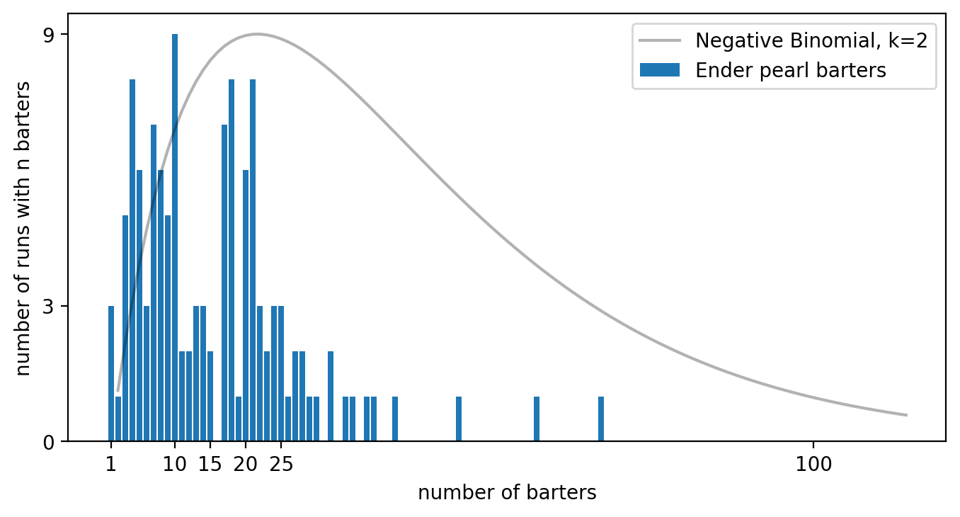
Fig. 13 The number of barters performed during a speedrun, for sessions that had zero to two successful barters, according to the Minecraft Speeedrunning Team.
The data does show a bit of a cliff at the \(n = 20\) mark, but it’s more of a mesa with tonnes of debris at the base. There isn’t a hard stopping time, it looks more like players trail off after that time. There’s also an unusual number of runs that end around \(n = 10\), much more than we’d expect from a Negative Binomial, and an unusual lack of runs in the teens. This might be due to where players decide to stop.
r_pearl = 20/423

x       = np.arange(1,int(all_pearl_barters['n'].max()))

fig = plt.figure(figsize=(8, 4), dpi=dpi, facecolor='w', edgecolor='k')
axs = fig.subplots(3, 1)

for k in range(3):

    # we only care about a specific k
    mask = all_pearl_barters['k'] == k
    pearl_x = all_pearl_barters[ mask ]['n'].unique()
    pearl_y = [all_pearl_barters[ mask & (all_pearl_barters['n'] == n) ]['n'].count() for n in pearl_x]

    # colour helps separate these
    colour    = [.3,.3,.3]
    colour[k] = .6
    axs[k].bar( pearl_x, pearl_y, label=f'k={k}', color=colour )

    # add the negative binomial
    nbinom_y = nbinom(2, r_pearl).pmf( x )
    axs[k].plot( x+2, nbinom_y/np.max(nbinom_y)*np.max(pearl_y), '-k', alpha=0.3 )

    axs[k].set_xticks([1,10,15,20,25,100])
    axs[k].set_yticks([0,3,6])
    axs[k].legend()

# we only need one label
axs[1].set_ylabel( 'frequency' )
axs[2].set_xlabel( 'number of barters in a run' )

fig_show( fig, 'fig:barters_by_k' )
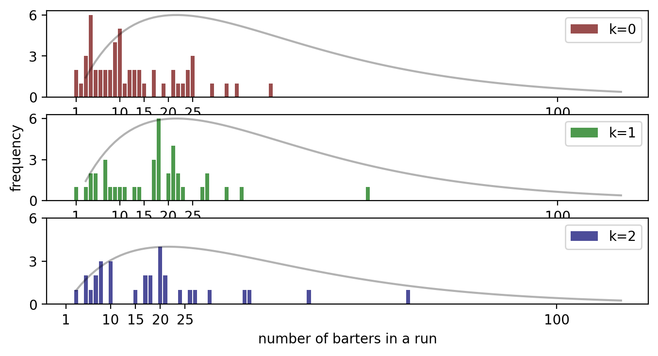
Fig. 14 The number of barters performed during a speedrun, for sessions that had zero to two successful barters, according to the Minecraft Speeedrunning Team. Each count of successful barters is plotted separately.
The number of barters differs significantly for speedrunners that had zero Ender pearl barters. This makes sense if they are time or resource limited, as the odds of getting two successful barters before the limit is reached diminishes with each barter performed. Interestingly, the distribution bears a vague resemblance to the Exponential, implying that speedrunners have a fixed probability of quitting after each barter. The resemblance is not perfect, though, as the peak number of barters is \(n = 4\) instead of \(n = 1\), the latter being what we expect from the Exponential distribution. This suggests speedrunners wait a few barters to see if they’ll earn any Ender pearls before considering dropping out. A better strategy would be to calculate when the probability of earning two pearl barters before running out of time or gold drops below a threshold and always bartering until that point, which gives a very different distribution.
The distributions for \(k = 1\) and \(k = 2\) are remarkably similar, though the former peaks earlier. This is more in line with the improved strategy outlined above, with further evidence coming from the lack of runs for \(k = 1\) and \(8 \le n \le 16\). There are not a lot of datapoints to work from, however, so these could be false patterns.
Our simulation for Ender pearl barters must take as much of the above into account as possible. I propose the following:
Draw a maximum number of barters to perform, \(n_\text{max}\), from the observed distribution of \(n\) for \(k < 3\).
Draw a number of successful barters, \(k_\text{max}\), from \(\text{Binom}( n_\text{max}, r )\), where \(r \in \{r_\text{fair}, r_\text{cheat} \}\).
Draw a number of barters to perform, \(n_\text{success}\), from \(\text{NegBinom}( 2, r )\).
If \(n_\text{success} < n_\text{max}\), use \((n_\text{success}, 2)\) as the results of this run. Otherwise, use \((n_\text{max}, k_\text{max}).\)
Notice that \(k\) is never checked, so \(k_\text{max} > 2\) is possible. This is a better match for the observed data, as sometimes speedrunners do have more than two Ender pearl barters per run. For the cheating player, we will use \(r_\text{cheat} \approx {}\) 6.383%. All values besides \(r_\text{fair}\) are identical with the previous simulation.
random  = np.random.default_rng(64)

r_fair    = 20/423 ; glue( 'sim_pearl_r_fair', r_fair*100, display=False )
r_cheat_h = 27/423 ; glue( 'sim_pearl_r_cheat_h', r_cheat_h*100, display=False )
count     = 200   ; glue( 'sim_pearl_count', count, display=False )
clones    = 16    ; glue( 'sim_pearl_clones', clones, display=False )
a_prior, b_prior   = prior(r_fair, 4)

# set up n_max
choices_n = np.array( all_pearl_barters[all_pearl_barters['k'] < 3]['n'].unique(), dtype='int64' )
weights_n = [all_pearl_barters[(all_pearl_barters['k'] < 3) & (all_pearl_barters['n'] == n)]['n'].count() \
              for n in choices_n]
weights_n = weights_n / np.sum(weights_n)

# draw n_max, k_max, and n_success for the cheater
vec_cheat_n_binom = random.choice( choices_n, p=weights_n, size=(clones,count) )
vec_cheat_k_binom = random.binomial( vec_cheat_n_binom, r_cheat_h )
vec_cheat_n_nbinom = random.negative_binomial( 2, r_cheat_h, size=(clones,count) ) + 2

# merge the two via vectorization
mask = vec_cheat_n_nbinom < vec_cheat_n_binom
vec_cheat_k = 2*mask + vec_cheat_k_binom*(1-mask)
vec_cheat_n = np.minimum( vec_cheat_n_nbinom, vec_cheat_n_binom )

# wash-rinse-repeat for the fair player
vec_fair_n_binom = random.choice( choices_n, p=weights_n, size=(clones,count) )
vec_fair_k_binom = random.binomial( vec_fair_n_binom, r_fair )
vec_fair_n_nbinom = random.negative_binomial( 2, r_fair, size=(clones,count) ) + 2

mask = vec_fair_n_nbinom < vec_fair_n_binom
vec_fair_k = 2*mask + vec_fair_k_binom*(1-mask)
vec_fair_n = np.minimum( vec_fair_n_nbinom, vec_fair_n_binom )

# calculate cumulative sums
sum_fair_k = np.cumsum( vec_fair_k, axis=1 )
sum_fair_n = np.cumsum( vec_fair_n, axis=1 )
sum_cheat_k = np.cumsum( vec_cheat_k, axis=1 )
sum_cheat_n = np.cumsum( vec_cheat_n, axis=1 )

fig = plt.figure(figsize=(8, 4), dpi=dpi, facecolor='w', edgecolor='k')

x = np.arange(1,count+1)
for idx in range(clones):
    y = [BF_H_fair_H_cheat(sum_cheat_k[idx][i], sum_cheat_n[idx][i], r_fair, a_prior, b_prior) for i in range(count)]
    if idx == 0:
        plt.plot( x, y, '-r', label=f'cheater (r={r_cheat_h:.3f})' )
    else:
        plt.plot( x, y, '-r', alpha=0.1 )

    y = [BF_H_fair_H_cheat(sum_fair_k[idx][i], sum_fair_n[idx][i], r_fair, a_prior, b_prior) for i in range(count)]
    if idx == 0:
        plt.plot( x, y, '-k', label=f'fair (r={r_fair:.3f})' )
    else:
        plt.plot( x, y, '-k', alpha=0.1 )

plt.plot( x, [1 for v in x], '--g', label='break even' )

plt.xlabel("rounds")
plt.xticks([1,count])
plt.ylabel('H_fair / H_cheat')
plt.yscale("log")

plt.legend()
fig_show( fig, 'fig:sim_pearl_duo' )
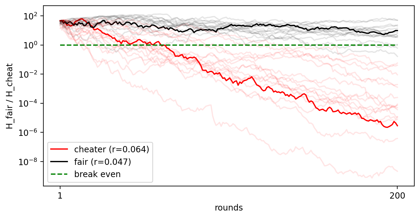
Fig. 15 The behaviour of this Bayes Factor for 16 clones of a player who modified their Ender pearl barter rate to be \(r_\text{cheat} \approx {}\) 6.383%, versus clones of a player who has not (\(r_\text{fair} \approx {}\) 4.728%).
The resulting simulation has a number of interesting properties. The cheater shows a similar descent to the previous figure, and yet as a proportion the level of cheating is more blatant. This is likely due to a combination of two things. Intuitively, it seems obvious that the rate of rare events would be more difficult to estimate than more common ones. As a consequence, though, it must also be difficult to estimate the frequency of very common events; if it was not, then we could switch from tracking when rare events do occur to when they do not and achieve a better estimate. This implies that the easiest event rate to track is neither common nor rare, when the rate of the event occurring matches the rate of it not occurring. That is \(r = \frac 1 2\), the rate of Blaze rod drops, so by this argument the lower rate of Ender pearl barters must make them more difficult to estimate. This intuition can be placed on firmer ground via Information theory.
It also should be noted that my prior for Ender pearl barters is fairly strong. My scale 4 prior for Blaze rod drops is mathematically equivalent to a Bayes/Laplace prior with six “phantom” observations added that precisely match the expected drop rate. The scale 4 prior for Ender pearl drops is equivalent to Bayes/Laplace with three successful Ender pearl drops observed and slightly more than 81 failed attempts. With so many phantom observations, overcoming the latter prior’s weight requires either many more observations or a greater level of bias.
Another interesting property is that the fair player no longer follows the \(\sqrt{n}\) rule, and in fact their Bayes factors show a gradual decline over time. You might have assumed that since this simulation was the combination of Negative Binomial and Binomial distributions with the same rate, and the math showed that this Bayes factor worked equally well on both distributions, it should have worked for our simulation. In reality, the way we combined the two distributions together created a subtle bias in the underlying success rate, skewing it from \(\frac{20}{423}\). The PE report was right to worry about this possibility, even if got the details wrong.
At the same time, the behaviour of the cheater and fair player are clearly different. A skew may be present, but it is much smaller than the difference between the cheating and fair rate. This shows that a flawed model can still be useful if it sufficiently close to reality, and if its flaws can be bounded. This is another reminder of why control groups and validation are so important.