Real-World Results¶

With the above analysis in place, we’re ready to look at real world data.

Blaze Rod Drops¶

We will begin with the Blaze rod data. The MST report gathered data for five distinct random-seed any-percent Minecraft 1.16 speedrunners: Benex, Dream, Illumina, Sizzler, and Vadikus007.

# Execute this cell to install all dependencies. Apologies for the spam.

# If you're running this on your own computer, I recommend altering "install mpmath" 
#  to read "install --user mpmath", that way you don't need administrator access.
# On Colab, change "pip -q install" to "pip install", as otherwise you could miss a message
#  that you need to restart your runtime. If you don't restart, the code won't work.
# A few error messages are fine, I usually get one about mismatched versions and the code
#  still runs. 

!pip -q install mpmath myst_nb numpy pandas matplotlib scipy

from fractions import Fraction

from math import log,factorial
import matplotlib.pyplot as plt
from mpmath import mp
from myst_nb import glue

import numpy as np

import pandas as pd
from scipy.optimize import differential_evolution
from scipy.stats import beta,binom,nbinom


dpi         = 200  # change this to increase/decrease the resolution charts are made at
book_output = True ### changing this to False will allow you to view the plots in a Jupyter notebook

def fig_show( fig, name ):
    """A helper to control how we're displaying figures."""
    global book_output
    
    if book_output:
        glue( name, fig, display=False )
        plt.close();
    else:
        fig.show()

# missing "simple_bernoulli_bf.py"? Uncomment this line to grab it from the repository
# !wget -c "https://raw.githubusercontent.com/hjhornbeck/bayes_speedrun_cheating/main/simple_bernoulli_bf.py"

from simple_bernoulli_bf import prior, posterior_H_fair, BF_H_fair_H_cheat

# missing the data files? Uncommenting and running this cell might retrieve them

# !mkdir data
# !wget -cP data "https://raw.githubusercontent.com/hjhornbeck/bayes_speedrun_cheating/main/data/blaze.benex.tsv"
# !wget -cP data "https://raw.githubusercontent.com/hjhornbeck/bayes_speedrun_cheating/main/data/blaze.dream.tsv"
# !wget -cP data "https://raw.githubusercontent.com/hjhornbeck/bayes_speedrun_cheating/main/data/blaze.illumina.tsv"
# !wget -cP data "https://raw.githubusercontent.com/hjhornbeck/bayes_speedrun_cheating/main/data/blaze.sizzler.tsv"
# !wget -cP data "https://raw.githubusercontent.com/hjhornbeck/bayes_speedrun_cheating/main/data/blaze.vadikus007.tsv"

colours = ['b', 'g', 'r', 'c', 'm', 'y', 'k']  # makes colouring some of the following easier
colours = colours + colours                    # double-up to allow for extra data

blaze_players = ['benex','dream','illumina','sizzler','vadikus007']

blaze_rods = {p:pd.read_csv(f'data/blaze.{p}.tsv',sep="\t") for p in blaze_players}


# Want to add your own data? The easiest way is to gather your data, then edit and uncomment this:

# vec_n = [12, 11, 16, 10, 13, 11, 5, 4, 1, 14]
# vec_k = [ 6,  7,  8,  7,  8,  8, 5, 3, 1,  8]
# blaze_rods['NAME'] = pd.DataFrame( {'n':vec_n, 'k':vec_k} )

blaze_rods['dream'].set_index('n').transpose()

n	12	11	16	10	13	11	5	4	1	14	...	9	10	15	10	15	11	9	10	9	9
k	6	7	8	7	8	8	5	3	1	8	...	8	6	8	7	7	7	7	7	7	8

1 rows × 33 columns

We’ll use the same charts as with the simulation, where the Bayes factor is updated as new data is added. This responds to a critique of the PE report: if the same trend is observed regardless of whether or not the last datapoint is dropped, we can be reasonably confident it was not an artifact of our stopping point.

As promised, we will determine the influence of the prior by varying the scale parameter. My preferred value of 4 will be scaled by values ranging between \(\frac 1 3\) and 3. The higher multiplier will “tug” the posterior towards the default hypothesis, while the lower gives the data more power to shape the posterior.

r_fair = Fraction(1,2)

# only the two extremes need to be explicitly calculated
priors = [prior( r_fair, scale ) for scale in [Fraction(4,3), 4, 12]]


fig = plt.figure(figsize=(8, 4), dpi=dpi, facecolor='w', edgecolor='k')

max_count = 0  # note the largest number of runs by a player
xtics = set()  # we'd like some fancy X-axis ticks

for i,p in enumerate(blaze_rods.keys()):
    
    # update the above variables
    count = len(blaze_rods[p])
    if count > max_count:
        max_count = count
    xtics.add( count )
       
    x     = np.arange(1, count+1)
    sum_n = np.cumsum( blaze_rods[p]['n'] )
    sum_k = np.cumsum( blaze_rods[p]['k'] )

    if p == 'dream':
        alpha = 1
    else:
        alpha = 0.3

    y = [BF_H_fair_H_cheat(sum_k[i], sum_n[i], r_fair, *priors[1]) for i in range(count)]
    plt.plot( x, y, '-', label=p, c=colours[i], alpha=alpha )
    
    y_low = [BF_H_fair_H_cheat(sum_k[i], sum_n[i], r_fair, *priors[0]) for i in range(count)]
    y_hig = [BF_H_fair_H_cheat(sum_k[i], sum_n[i], r_fair, *priors[2]) for i in range(count)]
    plt.fill_between( x, [float(v) for v in y_low], [float(v) for v in y_hig], \
                     alpha=0.2*alpha, color=colours[i] )

# build the fancy ticks
xtics.discard( max_count )
xtics = [ (x >> 1) << 1 for x in xtics]
xtics.extend( [ ((x >> 1) + 1) << 1 for x in xtics if x + 1 < max_count] )
xtics.extend( [1,max_count] )


x = range(1,max_count+1)
plt.plot( x, [1 for v in x], '--k', label='break even' )

plt.xlabel("run")
plt.xticks( list(xtics) )
plt.ylabel('H_fair / H_cheat')
plt.yscale("log")

plt.legend()
fig_show( fig, 'fig:data_blaze' )

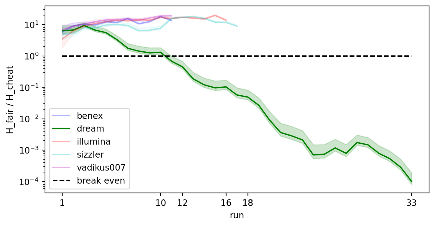
Fig. 16 The behaviour of this Bayes Factor for the Blaze rod drops of serveral Minecraft 1.16 speedrunners, using data from the MST report.¶

The Bayes factor for Dream’s Blaze rod drop rate behaves differently from other Minecraft speedrunners. It drops like the cheating players from the Blaze rod simulation, but at a much sharper rate. Removing the last datapoint does not impact that trend. There is evidence the Bayes factor of two other runners are curving back towards the 1:1 odds line, but that’s still consistent with random fluctuations due to normal gameplay. It might also indicate Blaze rods do not follow the Binomial or Negative Binomial distributions, but we’d need quite a bit more data to be sure.

The choice of prior doesn’t have a significant impact, but it should be noted the log scaling downplays the difference between the priors. The Bayes factor for Dream’s round thirty-three using the scale 4 prior is half the size of the BF for the scale 12 prior, for instance.

r_fair         = Fraction(1,2)
sum_n          = blaze_rods['dream']['n'].sum()
sum_k          = blaze_rods['dream']['k'].sum()
dream_blaze_bf = BF_H_fair_H_cheat( sum_k, sum_n, r_fair, *prior(r_fair,4) )

print( f"The Bayes factor for Dream's Blaze rod rate, over all his rounds and with the scale 4 prior," + \
       f" is about {mp.nstr(dream_blaze_bf,3)}", end='' )

if dream_blaze_bf < 1:
    print( f", or 1:{int(mp.fdiv(1,dream_blaze_bf)):,}." )
else:
    print( "." )

The Bayes factor for Dream's Blaze rod rate, over all his rounds and with the scale 4 prior, is about 0.000101, or 1:9,930.

The resulting Bayes factor is roughly equivalent to the average golfer landing a hole in one on their next shot. In comparison, the equivalent p-value in the MST report is \(4.72 \times 10^{-11}\). Setting aside the different interpretations of both numbers, that’s a difference of seven orders of magnitude. This seems to bear out the assertion that Bayesian statistics is inherently more sluggish to respond to the evidence.

The PE report puts the probability of fair play at \(3 \times 10^{-8},\) however. Why do two Bayesian analyses come to two very different results? The PE report analyzed Dream’s drop rate by calculating a grid of probabilities ranging from \(\frac 1 2\) to \(\frac 9 {10}\), then taking the result for \(r_\text{blaze} = \frac 1 2\) as the probability of fair play (pg. 10). This is analogous to the idealized dart board, which by necessity will lead to more extreme values. By integrating over an area, my definition of both \(H_\text{fair}\) and \(H_\text{cheat}\) account for the random fluctuations we would expect from random data, which necessarily waters down the probabilities of each. The PE report also does not factor in the probability of \(H_\text{cheat}\). If that hypothesis is unlikely, then the relative likelihood of \(H_\text{fair}\) is boosted proportionately.

As nice as the Bayes factor chart is, it only tells us the relative probabilities of \(H_\text{fair}\) to \(H_\text{cheat}\). It gives no indication of what the most credible drop rate was. We can derive that by charting the posteriors for each player and noting the mean values. I’ll again vary the prior to observe how the posterior changes.

r_fair = Fraction(1,2)

fig = plt.figure(figsize=(8, 4), dpi=dpi, facecolor='w', edgecolor='k')

dream_mean = 0 

# we can't get away with just doing the extremes. Instead, spam priors!
priors = [prior( r_fair, scale ) for scale in np.exp(np.linspace( np.log(4/3), np.log(12), 32 ))]
a_prior, b_prior = prior( r_fair, 4 )

x_limits = [.4, .8]
x = np.linspace( *x_limits, 512 )
for i,p in enumerate(blaze_rods.keys()):

    sum_n = np.sum( blaze_rods[p]['n'] )
    sum_k = np.sum( blaze_rods[p]['k'] )
    
    if p == 'dream':
        alpha = 1
    else:
        alpha = 0.3

    plt.plot( x, beta.pdf( x, float(a_prior + sum_k), float(b_prior + sum_n - sum_k) ), \
             '-', label=p, c=colours[i], alpha=alpha )
    for pr in priors:
        plt.plot( x, beta.pdf( x, float(pr[0] + sum_k), float(pr[1] + sum_n - sum_k) ), \
             '-', alpha=0.1*alpha, c=colours[i] )

    # plot the mean
    plt.axvline( (a_prior + sum_k)/(a_prior + b_prior + sum_n), c=colours[i], alpha=0.3*alpha )
    
    if p == 'dream':
        dream_mean = (a_prior + sum_k)/(a_prior + b_prior + sum_n)
    
plt.xlabel("rate")
plt.xlim( x_limits )
plt.xticks( [.4, .5, .55, float(dream_mean), .8] )
plt.ylabel('likelihood')
plt.yticks([])

plt.legend()
fig_show( fig, 'fig:data_blaze_pos' )

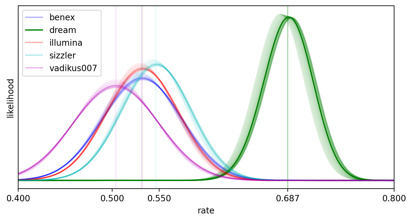
Fig. 17 The posterior distribution for the Blaze rod drops of several Minecraft 1.16 speedrunners, using data from the MST report. Vertical lines represent the mean of the posterior with the scale 4 prior.”,¶

The posterior distributions of other Minecraft players cluster on the generous side of 50:50 odds. Sizzler is the largest outlier, with the mean of his posterior approaching 55%, but even in their case a substantial amount of credence is present for \(r_\text{blaze} \le \frac 1 2\). Dream again stands alone, with the posterior’s mean drop rate above \(\frac 2 3\) and almost no credence around \(\frac 1 2\). This is similar to the PE report’s estimate of “around 0.7” (pg. 10). Strengthening the prior clusters the credence more tightly around \(r_\text{blaze} = \frac 1 2\), but there is sufficient data to make the effect subtle at best.

r_fair           = Fraction(1,2)
sum_n            = blaze_rods['dream']['n'].sum()
sum_k            = blaze_rods['dream']['k'].sum()
a_prior, b_prior = prior(r_fair,4)

bounds = [.025, .16, .5, .84, .975]
intervals = beta.ppf( bounds, float(a_prior + sum_k), float(b_prior + sum_n - sum_k) )
glue( 'data_blaze_intervals_low', intervals[0], display=False )
glue( 'data_blaze_intervals_high', intervals[4], display=False )
glue( 'interval_width', (bounds[4]-bounds[0])*100, display=False )

print( "Given the above data and prior, about two-thirds of our credence for Dream's Blaze rod rate\n" + \
      f"  is in the interval [{intervals[1]:.3f}, {intervals[3]:.3f}], while about 95% is between " + \
      f"[{intervals[0]:.3f}, {intervals[4]:.3f}]. The median is roughly {intervals[2]:.3f}." )

Given the above data and prior, about two-thirds of our credence for Dream's Blaze rod rate
  is in the interval [0.661, 0.713], while about 95% is between [0.635, 0.737]. The median is roughly 0.687.

When estimating a parameter, it’s quite common to generate confidence or credible intervals for it. Those can reiterate some of the problems of p-values, such as what the interval means or what counts as extreme,[MHR+16] plus there is no hard and fast rule on how much credence should be contained within the interval. The traditional value of 95% can be sensitive to extreme data, so I prefer \(\frac 2 3\). If you insist on some sort of credible interval calculation, then the 95.0% credible interval for Dream’s Blaze rod drop rate is [0.635, 0.737].

Ender Pearl Barters¶

We have two sources of data for Ender pearls. The MST report collected bartering data for five runners including Dream, and Dream himself provided a spreadsheet with more data. Accessing that spreadsheet requires giving Dream or a third party my Google account information, so I instead opted to use the data listed in Appendix A of the PE report. I’ve labelled this second source “dream_before”, as it covers a period before Dream took time off of Minecraft speed runs. The MST’s data on Dream is labelled “dream_after”, for similar reasons.

This provides us with an easy way to consider which, if any, of the above cheating scenarios apply.

If Dream cheated, and if he altered his barter rate from the start, we would expect the Bayes factor of both datasets to act like cheating players from the simulation and both posteriors to have little credence around \(r_\text{blaze} = \frac{20}{423}\).
If Dream cheated, but only after he took some time off, we would expect the BF of the “before” set to behave like any other Minecraft speedrunner while the BF of the “after” acts like a cheating player. The posteriors would, respectively, cluster around \(\frac{20}{423}\) and higher than it.
If Dream cheated, but craftily reduced his barter rate to hide it, we would expect the BF of both datasets to act like cheating players. The posteriors would, respectively, cluster below \(\frac{20}{423}\) and above it.

Scenario 1 has already been ruled out by the PE report, as it notes the additional data reduces the probability of Dream cheating (pg. 13).

# missing the data files? Uncommenting and running this cell might retrieve them

# !mkdir data
# !wget -cP data "https://raw.githubusercontent.com/hjhornbeck/bayes_speedrun_cheating/main/data/bartering.benex.tsv"
# !wget -cP data "https://raw.githubusercontent.com/hjhornbeck/bayes_speedrun_cheating/main/data/bartering.dream_before.tsv"
# !wget -cP data "https://raw.githubusercontent.com/hjhornbeck/bayes_speedrun_cheating/main/data/bartering.dream_after.tsv"
# !wget -cP data "https://raw.githubusercontent.com/hjhornbeck/bayes_speedrun_cheating/main/data/bartering.illumina.tsv"
# !wget -cP data "https://raw.githubusercontent.com/hjhornbeck/bayes_speedrun_cheating/main/data/bartering.sizzler.tsv"
# !wget -cP data "https://raw.githubusercontent.com/hjhornbeck/bayes_speedrun_cheating/main/data/bartering.vadikus007.tsv"

colours = ['b', 'g', 'r', 'c', 'm', 'y', 'k']  # makes colouring some of the following easier
colours = colours + colours                    # double-up to allow for extra data

pearl_players = ['benex','dream_before','dream_after','illumina','sizzler','vadikus007']

bartering  = {p:pd.read_csv(f'data/bartering.{p}.tsv',sep="\t") for p in pearl_players}
    
    
# Want to add your own data? The easiest way is to gather your data, then edit and uncomment this:

# vec_n = [12, 11, 16, 10, 13, 11, 5, 4, 1, 14]
# vec_k = [ 6,  7,  8,  7,  8,  8, 5, 3, 1,  8]
# bartering['NAME'] = pd.DataFrame( {'n':vec_n, 'k':vec_k} )
    
bartering['dream_after'].set_index('n').transpose()

n	22	5	24	18	4	1	7	12	26	8	...	2	13	10	10	21	20	10	3	18	3
k	3	2	2	2	0	1	2	5	3	2	...	0	1	2	2	2	2	2	1	2	2

1 rows × 22 columns

r_fair = Fraction(20,423)
priors = [prior( r_fair, scale ) for scale in [Fraction(4,3), 4, 12]]

# same old, same old
fig = plt.figure(figsize=(8, 4), dpi=dpi, facecolor='w', edgecolor='k')

max_count = 0
xtics = set()

for i,p in enumerate(bartering.keys()):
    
    count = len(bartering[p])
    if count > max_count:
        max_count = count
    xtics.add( count )
        
    x     = np.arange(1, count+1)
    sum_n = np.cumsum( bartering[p]['n'] )
    sum_k = np.cumsum( bartering[p]['k'] )

    if p == 'dream_after':
        alpha = 1
    else:
        alpha = 0.3

    y = [BF_H_fair_H_cheat(sum_k[i], sum_n[i], r_fair, *priors[1]) for i in range(count)]
    plt.plot( x, y, '-', label=p, c=colours[i], alpha=alpha )
    
    y_low = [BF_H_fair_H_cheat(sum_k[i], sum_n[i], r_fair, *priors[0]) for i in range(count)]
    y_hig = [BF_H_fair_H_cheat(sum_k[i], sum_n[i], r_fair, *priors[2]) for i in range(count)]
    plt.fill_between( x, [float(v) for v in y_low], [float(v) for v in y_hig], \
                     alpha=0.1*alpha, color=colours[i] )

# build the fancy ticks
xtics.discard( max_count )
xtics = [ (x >> 1) << 1 for x in xtics]
xtics.extend( [ ((x >> 1) + 1) << 1 for x in xtics if x + 1 < max_count] )
xtics.extend( [1,max_count] )

    
x = range(1,max_count+1)
plt.plot( x, [1 for v in x], '--k', label='break even' )

plt.xlabel("run")
plt.xticks( xtics )

plt.ylabel('H_fair / H_cheat')
plt.yscale("log")

plt.legend()
fig_show( fig, 'fig:data_pearl' )

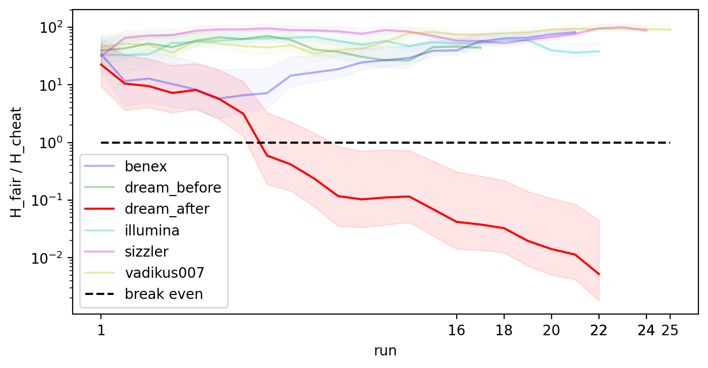
Fig. 18 The behaviour of this Bayes Factor for Ender pearl barters, from both reports.¶

This time there’s less certainty. The same pattern is present, but only for Dream after he returned to random-seed any-percent Minecraft 1.16. The other speedrunners and Dream’s earlier runs behave more like fair players, and generally follow the \(\sqrt{n}\) curve. Benex’s first six rounds do show a downward trajectory, but their later data restores the behaviour of a fair player. This provides mild evidence for Scenario 3 cheating, but the magnitudes involved are small enough that it can also be explained by unusually good luck. On the whole, for Dream, Scenario 2 is the most likely case.

The choice of prior has a much stronger on the final outcome here than it did before, and the probabilities are about two orders of magnitude higher. As mentioned, the rarity of Ender pearl barters relative to Blaze rod drops makes their rate harder to estimate, and the stronger prior for barters gives it a greater influence over the posterior.

sum_n          = np.sum( bartering['dream_after']['n'] )
sum_k          = np.sum( bartering['dream_after']['k'] )
dream_pearl_bf = BF_H_fair_H_cheat( sum_k, sum_n, r_fair, *prior(r_fair,4) )

print( f"The Bayes factor for Dream's post-break Ender pearl barters, over all his rounds and with the scale 4 prior," + \
       f" is {mp.nstr(dream_pearl_bf,3)}", end='' )
if dream_pearl_bf < 1:
    print( f", or about 1:{int(mp.fdiv(1,dream_pearl_bf)):,}." )
else:
    print( "." )

The Bayes factor for Dream's post-break Ender pearl barters, over all his rounds and with the scale 4 prior, is 0.00523, or about 1:191.

With my scale 4 prior, the relative odds between \(H_\text{fair}\) and \(H_\text{cheat}\) are about the odds of a US citizen dying of an accidental poisoning. Alternatively, it’s more or less the odds of being born sometime during the first two days of June. A rare occurrence, certainly, but not that rare.

For comparison, the MST report put the p-value of this at \(8.04 \times 10^{-7}\), which differs by five orders of magnitude. The PE report gives the probability of fair play at \(3 \times 10^{-10}\) (pg. 11), but that number uses the same methodology as was used for Blaze rods and so the same criticisms apply.

fig = plt.figure(figsize=(8, 4), dpi=dpi, facecolor='w', edgecolor='k')

dream_mean = 0  # store Dream's mean value here
dream_means = list()

# fill_between doesn't give good output here. Instead, spam priors!
priors = [prior( r_fair, scale ) for scale in np.exp(np.linspace( np.log(4/3), np.log(12), 128 ))]
a_prior, b_prior = prior( r_fair, 4 )

x = np.linspace( 0, .2, 512 )
for i,p in enumerate(bartering.keys()):

    sum_n = np.sum( bartering[p]['n'] )
    sum_k = np.sum( bartering[p]['k'] )
    
    if p == 'dream_after':
        alpha = 1
    else:
        alpha = 0.3

    plt.plot( x, beta.pdf( x, float(a_prior + sum_k), float(b_prior + sum_n - sum_k) ), \
             '-', label=p, c=colours[i], alpha=alpha )
    for pr in priors:
        plt.plot( x, beta.pdf( x, float(pr[0] + sum_k), float(pr[1] + sum_n - sum_k) ), \
             '-', alpha=0.03*alpha, c=colours[i] )
        if p == 'dream_after':
            dream_means.append( (pr[0] + sum_k) / (pr[0] + pr[1] + sum_n) )

    plt.axvline( (a_prior + sum_k)/(a_prior + b_prior + sum_n), c=colours[i], alpha=0.3 )
    
    if p == 'dream_after':
        dream_mean = (a_prior + sum_k)/(a_prior + b_prior + sum_n)
    
plt.xlabel("rate")
plt.xlim( [0,.2] )
plt.xticks( [0, float(r_fair), float(dream_mean), .2] )
plt.ylabel('likelihood')
plt.yticks([])

plt.legend()
fig_show( fig, 'fig:data_pearl_pos' )

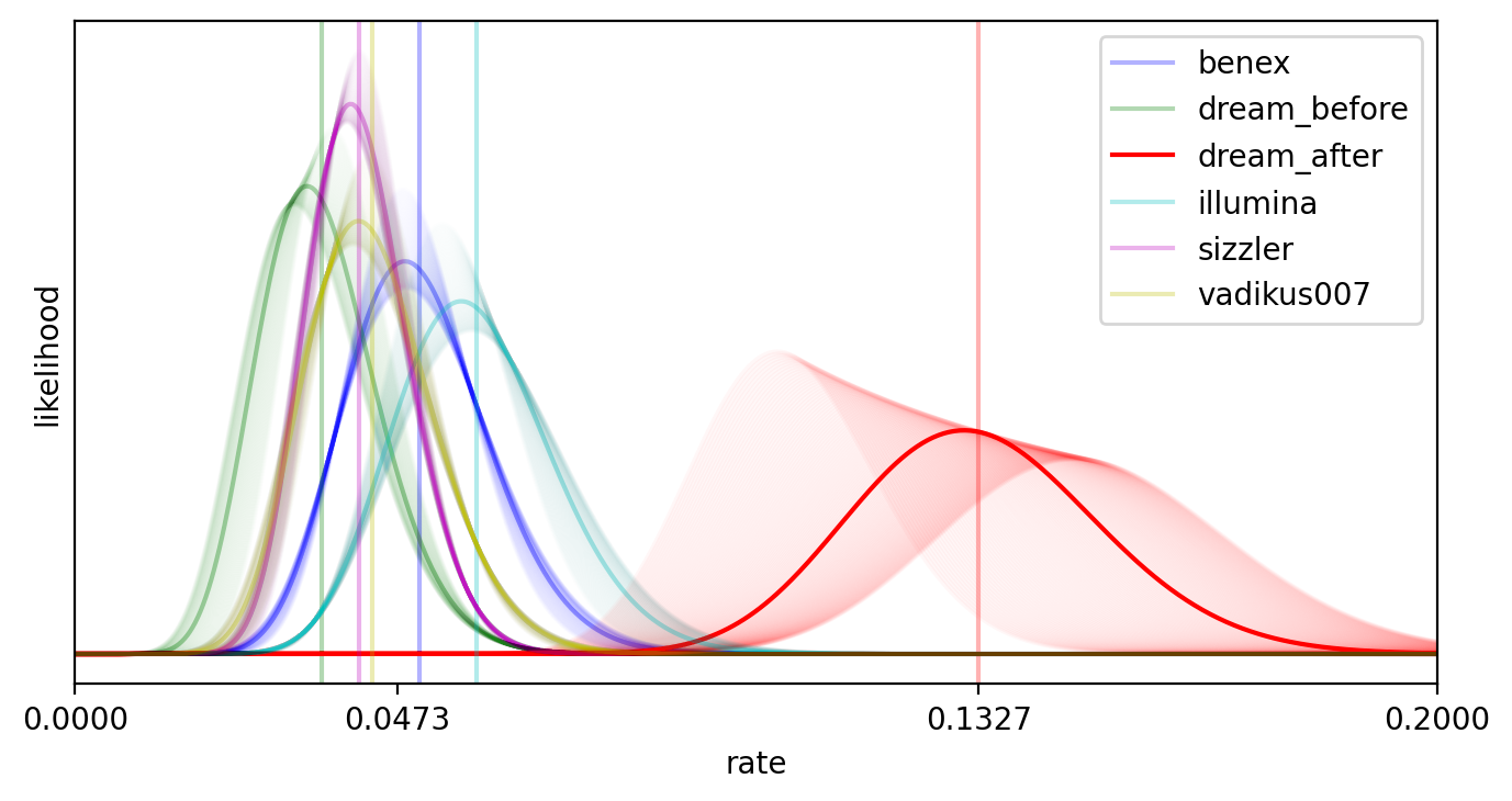
Fig. 19 The posterior distribution for the Ender pearl barters of several Minecraft 1.16 speedrunners, using data from both reports. Vertical lines represent the mean of the posterior for the scale 4 prior, and the effect of different priors is shown.¶

All but one sequence hovers around the expected rate of Ender pearl barters. The posterior for Dream’s performance before his break favours lower barter rates than all other runners, providing a little support for Scenario 3, but a non-trivial amount of credence is greater than the expected barter rate. Overall, Scenario 2 remains more likely. Dream’s post-break performance again is quite different from other speedrunners and even his own pre-break performance, but this time prior strength is a major factor. Even with the strongest prior, though, very little credence for Dream’s post-break barters is around the unaltered rate.

The mean value of Dream’s post-break performance is approximately three times larger than the expected rate, which again matches what the PE report observed (pg. 11).

r_fair           = Fraction(20,423)
sum_n            = bartering['dream_after']['n'].sum()
sum_k            = bartering['dream_after']['k'].sum()
a_prior, b_prior = prior(r_fair,4)

bounds = [.025, .16, .5, .84, .975]
intervals = beta.ppf( bounds, float(a_prior + sum_k), float(b_prior + sum_n - sum_k) )
glue( 'data_pearl_intervals_low', intervals[0], display=False )
glue( 'data_pearl_intervals_high', intervals[4], display=False )
glue( 'r_pearl', float(r_fair), display=False )

print( "Given the above data and prior, about two-thirds of our credence for Dream's Ender pearl barter rate\n" + \
      f"  is in the interval [{intervals[1]:.3f}, {intervals[3]:.3f}], while about 95% is between " + \
      f"[{intervals[0]:.3f}, {intervals[4]:.3f}]. The median is roughly {intervals[2]:.3f}." )

Given the above data and prior, about two-thirds of our credence for Dream's Ender pearl barter rate
  is in the interval [0.115, 0.151], while about 95% is between [0.099, 0.170]. The median is roughly 0.132.

A common heuristic is to see if the value we expect to see is contained within the interval, and invoke modus tollens if it is not. I do not endorse that, but if you disagree then I’ll simply note that the 95.0% credible interval is [0.0991, 0.1703], which does not include the unaltered Ender pearl barter rate of 0.0473%.

Combining Both Datasets¶

As mentioned earlier, Bayes factors are likelihoods and can thus be multiplied together. This allows us to generate a combined odds ratio for both datasets.

dream_combo_bf = mp.fmul( dream_blaze_bf, dream_pearl_bf )

print( f"The Bayes factor for both rates, over all of Dream's post-break rounds and with the scale 4 prior," + \
       f" is {mp.nstr(dream_combo_bf,3)}, or about 1:{int(mp.fdiv(1,dream_combo_bf)):,}." )

The Bayes factor for both rates, over all of Dream's post-break rounds and with the scale 4 prior, is 5.27e-7, or about 1:1,899,071.

The combined Bayes factor is quite low. To take an example, the median age of a Canadian in 2019 was about 41 years old. If we examine the relevant mortuary tables and extrapolate the odds of dying per year to the odds of dying per day, then we’d place four times more credence on a specific 41-year-old Canadian woman dying within 24 hours (about 1:472,632) than we would for \(H_\text{cheat}\) over \(H_\text{fair}\).

As unlikely as that is, it’s still seven orders of magnitude higher than the MST report’s “loose upper bound” on Dream’s success, which they declare is “almost certainly an overestimate” (pg. 22). After applying multiple corrections, the PE report concludes “there is a 1 in 100 million chance that a livestream in the Minecraft speedrunning community got as lucky this year on two separate random modes as Dream did in these six streams” (pg. 16), a number which is just about two order of magnitudes lower than what I calculate. The differences are entirely due to statistical methodology.

Did Dream Cheat? A Bayesian Analysis of a Bernoulli Process.

Real-World Results¶

Blaze Rod Drops¶

Ender Pearl Barters¶

Combining Both Datasets¶