Methodology
Given the flaws in both reports’ methodology, it is fair to ask what a better one looks like.
The Binomial and Negative Binomial Distributions
As the MST report shows, when a Blaze is killed it almost always drops either zero or one Blaze rod. Both outcomes are equally likely. These drops behave like a Bernoulli process:
Some algorithm or thing will “emit” one of two possible outputs, canonically labelled 0 and 1.
The choice of which value to emit cannot be predicted beforehand.
The current output does not depend on what’s been generated before or will be generated later.
As the number of values emitted becomes arbitrarily large, the ratio of zeros to ones comes arbitrarily close to a fixed value. That value does not change if we discard an arbitrary number of those outputs.
We can easily simulate that behaviour. Suppose I decided to collect Blaze rods for the first time, and set out to kill six Blazes. Since you can learn little from a single experiment, I do another four Blaze killing sprees.
# Execute this cell to install all dependencies. Apologies for the spam.

# If you're running this on your own computer, I recommend altering "install mpmath"
#  to read "install --user mpmath", that way you don't need administrator access.
# On Colab, change "pip -q install" to "pip install", as otherwise you could miss a message
#  that you need to restart your runtime. If you don't restart, the code won't work.
# A few error messages are fine, I usually get one about mismatched versions and the code
#  still runs.

!pip -q install mpmath myst_nb numpy pandas matplotlib scipy
from fractions import Fraction

from math import log,factorial
import matplotlib.pyplot as plt
from mpmath import mp
from myst_nb import glue

import numpy as np

import pandas as pd
from scipy.stats import beta,binom,nbinom

dpi         = 200  # change this to increase/decrease the resolution charts are made at
book_output = True # changing this to False will make it easier to view plots in a Jupyter notebook

def fig_show( fig, name ):
    """A helper to control how we're displaying figures."""
    global book_output

    if book_output:
        glue( name, fig, display=False )
        plt.close();
    else:
        fig.show()
# fixing the seed allows for perfect replication
random  = np.random.default_rng(8)

n = 6     # number of Blazes killed
c = 5     # number of runs to kill n Blazes

for experiment in range(c):
    results = random.choice( 2, size=n )
    [print("[Blaze rod] ", end='') if x==1 else print("[ nothing ] ", end='') for x in results]
    print( f"   total = {sum(results)}/{n}" )
[Blaze rod] [ nothing ] [ nothing ] [Blaze rod] [ nothing ] [ nothing ]    total = 2/6
[Blaze rod] [Blaze rod] [Blaze rod] [Blaze rod] [ nothing ] [ nothing ]    total = 4/6
[Blaze rod] [ nothing ] [ nothing ] [ nothing ] [ nothing ] [ nothing ]    total = 1/6
[Blaze rod] [ nothing ] [Blaze rod] [ nothing ] [Blaze rod] [ nothing ]    total = 3/6
[ nothing ] [ nothing ] [ nothing ] [ nothing ] [Blaze rod] [Blaze rod]    total = 2/6
I might calculate my odds of getting exactly three rods by multiplying the odds of getting a rod (50%) by itself three times, then multiply that by the odds of not getting a rod (50%) three times. If I carry on that logic for all other possible outcomes and sum them up, however, I find the total probability of all outcomes is \(7 \cdot (\frac 1 2)^6 = \frac{7}{64}.\) Those probabilities should sum to one, if I’ve defined a probability distribution.
The error in my logic is that I’ve failed to account for multiple identical outcomes. Two of the five runs shown above have two total successes, but both earn those successes in a different way. Conversely, there’s only a single way for one of my runs to earn a Blaze rod from every Blaze. To correctly calculate the probability of \(k\) drops when killing \(n\) Blazes, I need to also calculate the number of ways I could have earned those drops. As luck would have it, the math to do that is pretty easy.
where “!” is the factorial function, \(n! = n \cdot (n-1) \cdot (n-2) \cdot \dots \cdot 3 \cdot 2\). When I combine those two components, I get the Binomial distribution.
where \(n\) is the number of times the Bernoulli process is sampled, \(k\) is the number of 1’s emitted, and \(p\) is the probability of that Bernoulli process emitting a 1. For my toy example above, we find the odds for \(n = 6\), \(k = 3\), and \(p = \frac 1 2\) are not \(\frac 7 {64}\) but instead \(\frac 5 {16}\). If I carry that on for all seven values of \(k\) and sum the probabilities, they do indeed add up to one.
def binomial( n, k, p ):
    return Fraction(factorial(n), factorial(k)*factorial(n-k)) * (p**k) * ((1-p)**(n-k))

n = 6
p = Fraction(1,2)

total = sum( binomial(n, k, p) for k in range(n+1) )
print( f'The sum of probabilities of all possible k is {total}', end='' )
if total == Fraction(1,1):
    print( ', which means Binom(n,k,p) defines a probability distribution over k.')
else:
    print( '.' )
The sum of probabilities of all possible k is 1, which means Binom(n,k,p) defines a probability distribution over k.
Suppose I make one tweak to the above scenario, though. This time around I want to earn three Blaze rods, to allow me to craft the six Ender pearls I have in my inventory into six Eyes of Ender.
random  = np.random.default_rng(15)

k = 3     # number of Blaze rods needed
c = 5     # number of runs to earn k Blaze rods

for experiment in range(c):
    results = random.choice( 2, size=16 )
    while np.sum(results) < k:
        results = np.append( results, random.choice( 2, size=16 ) )
    n = np.sum( np.cumsum( results ) < k ) + 1
    [print("[Blaze rod] ", end='') if x==1 else print("[ nothing ] ", end='') for x in results[:n]]
    print( f"   total = {k}/{n}" )
[Blaze rod] [Blaze rod] [Blaze rod]    total = 3/3
[Blaze rod] [ nothing ] [ nothing ] [Blaze rod] [ nothing ] [Blaze rod]    total = 3/6
[ nothing ] [ nothing ] [ nothing ] [ nothing ] [ nothing ] [Blaze rod] [Blaze rod] [Blaze rod]    total = 3/8
[ nothing ] [Blaze rod] [Blaze rod] [Blaze rod]    total = 3/4
[Blaze rod] [ nothing ] [ nothing ] [ nothing ] [Blaze rod] [ nothing ] [Blaze rod]    total = 3/7
Before, I fixed the number of Blazes I killed, \(n\), as well as the odds of earning a Blaze rod, \(p\), so the only thing that could vary was the number of rods \(k\). Now with \(k\) and \(p\) fixed, \(n\) must be the one to vary. That part is obvious, but look carefully at the last Blaze I kill before quitting. Each and every time, it drops a Blaze rod. In hindsight that makes perfect sense: I’ve got no reason to continue killing Blazes after I earn my third rod, after all. In the process, though, I’ve placed some constraints on the number of ways to earn three Blaze rods. The math we invoked earlier to calculate the total number of combinations no longer works.
There is a way to fix it. Rather than consider the full \(n\) kills, let’s stop at the \(n-1\)-th kill. At this point, I have \(k-1\) Blaze rods. Since this is Bernoulli process, I have no idea that my next Blaze will net me a rod and I can exit this thought experiment. The \(n-1\)-th Blaze may or may not have dropped a rod, as of this point all possible ways to earn \(k-1\) rods via \(n-1\) Blazes are available. There’s only one way to earn that \(k\)-th rod on my \(n\)-th, so it doesn’t contribute any new combinations and the total number is \({n-1 \choose k-1}\) instead of \({n \choose k}\).
The probability of getting those rods still works, though. The odds of me getting \(k\) rods over \(n\) trials with success probability \(p\) does not change whether I stop based on \(n\) or \(k\). Combining this all together, we find the equation that describes the odds of \(n\) trials when trying to earn \(k\) successes with probability of success \(p\) is
This is known as the Negative Binomial distribution. While it’s closely related to the Binomial distribution, it is not identical.
Conjugate Priors
Remember when I mentioned in Missing Context that calculating the integrals necessary for Bayesian statistics “is impractical for all but the easiest problems?” Here’s one exception: let’s switch out the Bernoulli process for another that emits real numbers that have a Gaussian distribution. We know the variance of this process but not the mean value. How could we estimate it?
An obvious approach is to leverage the central limit theorem: grab a bunch of numbers from this process, calculate their average, and use that to be the best estimate. That doesn’t give us a degree of credence for that estimate, though, we’d prefer some sort of distribution to represent our credence for where the mean is. We can get that by generating a Gaussian distribution representing our credence for where the mean lies. It would be handy to be able to take in multiple values at once, and we can again use the central limit theorem to construct a Gaussian distribution representing the likelihood. We still need some sort of prior, but since we know the variance we can just use a diffuse Gaussian distribution based loosely on that and rely on the data to tug the posterior in the right direction.
Noting that both the prior and posterior are Gaussian distributions. You might have figured out this allows us to iteratively update our posterior: as more data comes in, we turn it into a Gaussian prior, apply the Gaussian likelihood function, and get back another Gaussian posterior. What you may not have figured out is that the math to update our posterior is trivially easy:
where \(\mu_n\) and \(\sigma_n\) are the mean and standard devation of \(\{x_1, x_2, \dots, x_n\}\) new observations.
When the prior and posterior of a model follow the same distribution, that prior is called a conjugate prior. These are oases of easy math in what is otherwise a Bayesian wasteland of tangled computations. If we can find a conjugate applicable to the Binomial and Negative Binomial, our analysis will be immensely simpler. The Gaussian example I used above is tempting, as the Gaussian distribution is often used as an approximation of the Binomial.
But there’s no need to approximate here: the Binomial distribution has a conjugate prior, the Beta distribution. Even better, the appropriate updating rule doesn’t require a fixed \(k\) or \(n\). This saves us from having to apply corrections for speed-runners that choose different Blaze rod quotas or happen to pick up Ender pearls outside of bartering. We will need to do some math to convert it to handle the Negative Binomial scenario, though.
The updating rule for the Beta conjugate prior is
where \(\Gamma(x)\) is the Gamma function. It is an extrapolation of factorials, such that \(n! = \Gamma(n+1)\) for any positive integer \(n\). Unlike factorials, though, the Gamma function can be applied to fractions, real numbers, and even complex numbers.
Now we need to decide which Beta distribution to use as a prior. Two options are commonly used, the Bayes/Laplace prior (\(\alpha = \beta = 1\)) and the Jeffreys prior (\(\alpha = \beta = \frac 1 2\)). The PE report uses the Bayes/Laplace prior, and as per my critique in Biased Priors I do not think it is appropriate here. The same reasoning applies to the Jeffreys prior; it groups the credence around \(p = 0\) and \(p = 1\), both of which are unlikely possibilities in the context of Blaze rod drops and Ender pearl barters.
fig = plt.figure(figsize=(8, 4), dpi=dpi, facecolor='w', edgecolor='k')

x = np.linspace(0,1,512)
plt.plot( x, beta.pdf(x, 1, 1), '-r', label='Bayes/Laplace Prior')
plt.plot( x, beta.pdf(x, .5, .5), '-b', label="Jeffrey's Prior" )

plt.ylabel("Likelihood")
plt.ylim([0,3])
plt.yticks([])

plt.xlabel("p")
plt.xticks([0, .5, 1])

plt.legend()
fig_show( fig, "fig:common_priors" )
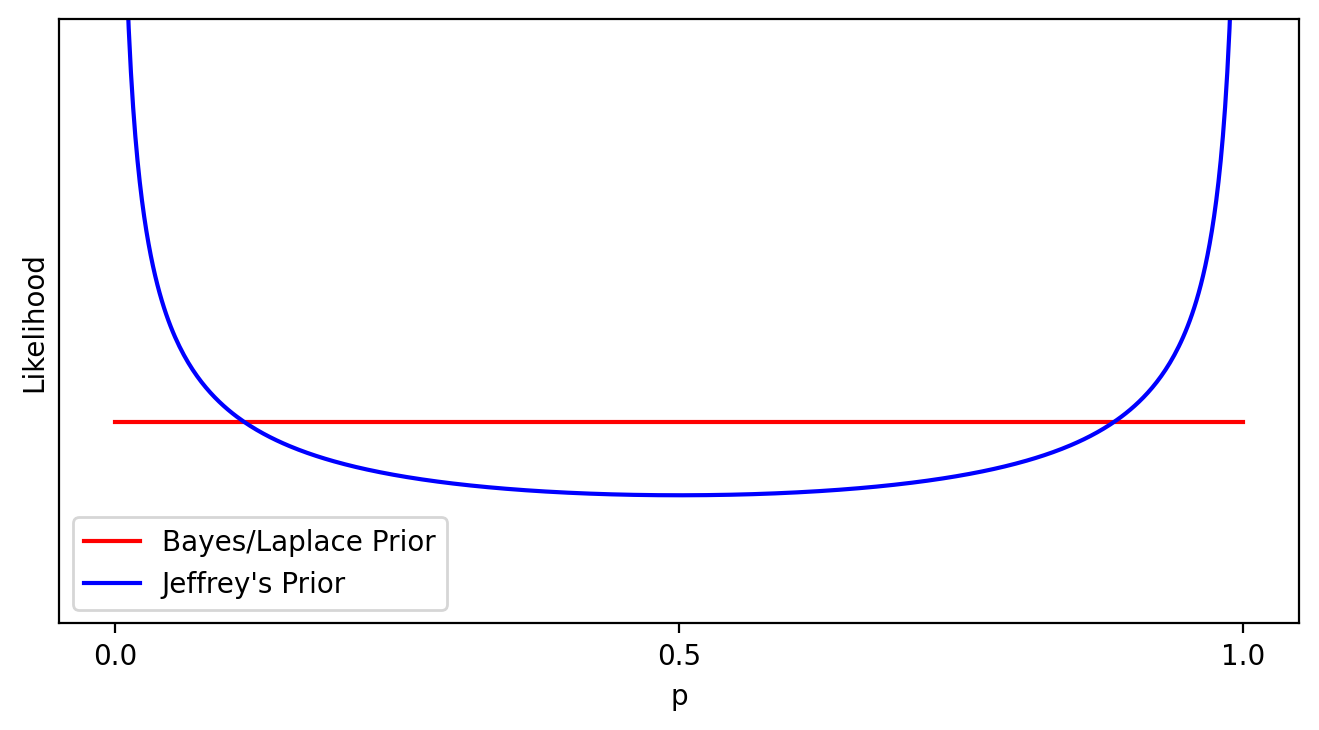
Fig. 1 The two most commonly used priors for the Beta distribution.
The prior I recommend instead places the bulk of the credence around the expected drop rate for each item, and spreads the remainder out according to a “strength” factor.
def prior(r, strength):
    """Generate an appropriate prior to be used during inference with a Beta conjugate prior.

    Parameters
    ----------
    r = The expected rate of item drops, assuming no modification of the game. Must be between 0 and 1.
    strength = A value to strengthen our credence around r. Higher values favour the hypothesis that
       someone played fairly, while lower values favour someone who cheated. Must be a positive real.

    Returns
    -------
    A tuple (alpha, beta) representing the Beta prior."""

    # ensure the proper values are given
    assert (r > 0) and (r < 1)
    assert strength > 0

    if r < .5:
        return (strength, strength*(1-r)/r)
    else:
        return (strength*(1-r)/r, strength)
fig = plt.figure(figsize=(8, 4), dpi=dpi, facecolor='w', edgecolor='k')
(ax1, ax2) = fig.subplots(1, 2)

x = np.linspace(0,1,512)

strengths = [2,4,8]
labels = [f'strength={strength}' for strength in strengths]
r_blaze = Fraction(1,2)
r_pearl = Fraction(20,423)

for i,strength in enumerate(strengths):

    blaze_prior = [float(x) for x in prior( r_blaze, strength )]
    ax1.plot(x, beta.pdf(x, *blaze_prior), '-', alpha=0.6, label=labels[i] )

    pearl_prior = [float(x) for x in prior( r_pearl, strength )]
    ax2.plot(x/5, beta.pdf(x/5, *pearl_prior), '-', alpha=0.6, label=labels[i] )


ax1.legend()
ax1.set_xticks([0,.5,1])
ax1.set_xlabel('drop rate, rods')
ax1.set_yticks([])
ax1.set_ylabel('likelihood')
ax1.axvline( r_blaze )

ax2.legend()
ax2.set_xticks([0,float(r_pearl),.1,.2])
ax2.set_xlabel('barter rate, pearls')
ax2.set_yticks([])
ax2.axvline( r_pearl )

fig_show( fig, "fig:sub_priors")
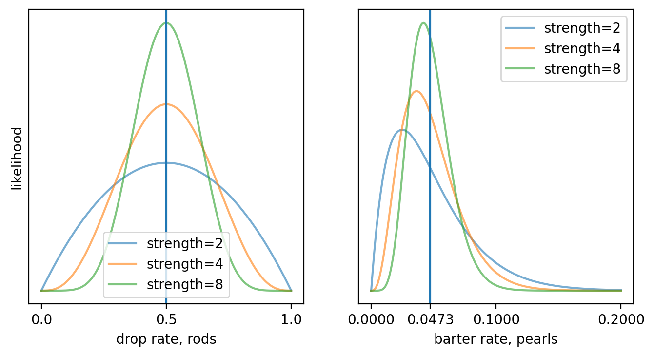
Fig. 2 Comparing my subjective priors for various strength factors. The vertical line is the expected or average value of the Bernoulli process.
These priors are all quite subjective, and ask you to make a judgment call on the appropriate strength value to use. I think 4 is a good compromise, but I’ll keep \(\alpha_\text{prior}\) and \(\beta_\text{prior}\) as free parameters. If you disagree with my subjective Beta prior, you’ll be free to substitute in any other. To double-check the effect of the strength parameter, I’ll also do a sensitivity analysis with the real-world data to get a better handle on the prior’s influence.
The apparent skew with the Ender pearl prior is because we are fixing the mean instead of the maximal likelihood. As we’ll be integrating across this prior, fixing the latter would bias us to assume the barter rate is higher.
The Posterior Distribution for the Binomial and Negative Binomial
We can now construct a posterior distribution for both the Binomial and Negative Binomial cases.
The updating rule of Equation (3) only works for one run of \(k\) successes via \(n\) trials, distributed according to the Binomial, but it is simple enough to extend for multiple runs. Define \(\vec n = \{n_1, n_2, \dots, n_c\}\) as a vector that contains the trial counts for all \(c\) runs, and \(\vec k = \{k_1, k_2, \dots, k_c\}\) as a vector for each success count. The resulting Beta posterior is
Equation (5) is a bit ugly to look at. One way to clean it up is to use different notation. The Taxicab norm is defined as
Since no value in \(\vec n\) or \(\vec k\) is negative, taking the absolute value has no effect. Note as well that
which, along with \(\|\vec k\|_1 + \|\vec n\|_1 - \|\vec k\|_1 = \|\vec n\|_1\), allows us to rewrite Equation (5) as
There’s no need to normalize Equation (8) to make it a probability distribution over \(p\), as
Or, in English, it was already normalized over \(p\).
That handles the case when \(\vec k\) and \(\vec n\) are taken from a Binomial distribution. What about the Negative Binomial case? Equation (2) shows the Negative Binomial is simply the Binomial times the probability of success. In theory, we could treat it the same as the Binomial case and apply some sort of correction to align it with the Negative Binomial. We have to be careful, though, as that equation also shows the Negative Binomial isn’t a probability distribution with respect to \(p\).
n = 6  # integrates to one with respect to p implies it does so regardless of what k and n are.
k = 3

# mp.quad() uses quadrature to numerically integrate. No math necessary on our side!
result = mp.quad( lambda p: p*binomial(n, k, p), (0,1) )
glue( 'nbinom_integral', float(result), display=False )

print( f'The integral of all possible p, for n={n} and k={k}, is {result}', end='' )
if result == Fraction(1,1):
    print( ', which means p*Binom(n,k,p) defines a probability distribution over p for at least that (n,k) pair.')
else:
    print( '.' )
The integral of all possible p, for n=6 and k=3, is 0.0714285714285714.
It is actually a probability distribution with respect to \(n\). We can fix that by normalizing it, and the best time to do so is after extending the updating rule. First, observe that
and secondly, remember that multiplication is commutative. This allows us to rearrange terms and write
We can tidy that up a bit, as \(p^a \cdot p^b = p^{a + b}\) and \(c - c = 0\).
To normalize Equation (12) according to \(p\), we only need to divide it by what it integrates to across \(p\).
Note that all the Gamma functions are constants, unaffected by any change in \(p\). As \(\int_x c \cdot g(x) = c \int_x g(x)\), we can pull them out of the integral. Since all the Gamma functions are identical across the numerator and denominator, they cancel out and we are left to evaluate
While this may seem daunting, remember that the Beta distribution integrates to 1 across \(p\). Thus we can rearrange Equation (9) to find
Equation (16) will be incredibly handy in future, but for now it allows us to finish normalizing Equation (12).
This is identical to Equation (8). The PE report was correct to raise the possibility that barters and drops do not follow the Binomial distribution (pg. 7), but an analysis that used the Negative Binomial instead would come to the same conclusion. The MST report is also incorrect when they state that the Binomial distribution is “a very good approximation” (pg. 10) for barters/drops, in reality it leads to the exact same outcome as assuming the Negative Binomial instead.
The posterior from Equation (18) is worth seeing in action. We’ll apply it to the last toy example from The Binomial and Negative Binomial Distributions, using the prior I defined earlier.
random  = np.random.default_rng(15)

k = 3     # number of Blaze rods needed
c = 5     # number of runs to earn k Blaze rods

sum_k = k * c  # we already know this
sum_n = 0

for experiment in range(c):
    results = random.choice( 2, size=16 )
    while np.sum(results) < k:
        results = np.append( results, random.choice( 2, size=16 ) )
    sum_n += np.sum( np.cumsum( results ) < k ) + 1

my_prior = prior(0.5, 4)

fig = plt.figure(figsize=(8, 4), dpi=dpi, facecolor='w', edgecolor='k')

x = np.linspace(0,1,512)
plt.fill_between( x, beta.pdf( x, my_prior[0] + sum_k, my_prior[1] + sum_n - sum_k), linestyle='-',
                label=f'prior + (sum_n = {sum_n}, sum_k = {sum_k})')

plt.plot( x, beta.pdf( x, my_prior[0], my_prior[1]), '-k', \
         label=f'prior (Beta({my_prior[0]:.1f},{my_prior[1]:.1f}))')
plt.axvline( 0.5, color='red' )

plt.xticks([0,.5,1])
plt.xlabel('p')

plt.yticks([])
plt.ylabel('likelihood')

plt.legend()
fig_show( fig, "fig:posterior_in_action")
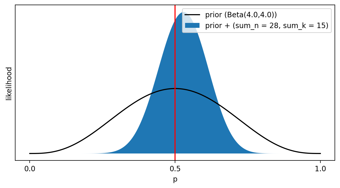
Fig. 3 The posterior for the last toy example of The Binomial and Negative Binomial Distributions, generated after adding the data to the previously-defined prior. The red vertical line coincides with the true drop rate.
The results are as expected. Our credence over the Blaze rod drop rate was fairly diffuse to begin with. Adding the simulation data grouped it more tightly together, making extremely low or high drop rates very unlikely. At the same time, the limited evidence allowed drop rates close to \(p = 0.5\) to remain very credible, and random variation kept the most likely drop rate of the posterior from matching the actual value. We’re more certain of the rate, but there’s still some wiggle room.
Defining Fairness
That last paragraph reveals a big problem. We have a mathematically-precise posterior distribution that contains our credence for all possible Blaze rod drop rates, but we’re not equally interested in all of them. Instead, we’re trying to translate the fuzzy concept of “fairness” into some subset of those rates and eyeballing how those specific rates perform within the posterior. The eyeballing part simply won’t do, as it doesn’t lay out all the underlying assumptions and relies on an estimate generated by a human being. We need to be much more rigorous, and come up with a mathematical definition of “did Dream cheat?” There is no obvious and unambiguous definition, but some definitions are better than others.
The easiest way to start is not by defining cheating, but instead defining fair play. We know unaltered Minecraft code sets the drop rate to 0.5, so why not define fairness by \(\text{Beta}( \alpha_\text{posterior}, \beta_\text{posterior}, 0.5)\)?
print( 'The likelihood I was playing fair in my simulation is' +
      f' {beta.pdf( 0.5, my_prior[0] + sum_k, my_prior[1] + sum_n - sum_k)} .')
The likelihood I was playing fair in my simulation is 4.490060385433022 .
That won’t work, if only because the output of the posterior is a likelihood, which isn’t normalized like a probability is. We need to find some way to scale or modify that value so it maps to something more meaningful to us.
But there’s a more subtle problem here. Imagine an idealized dart board, centred at the origin of a 2D Cartesian plane and with radius 1. Now pick a point on that dart board, and ask yourself the odds of an ideal dart hitting that point. The answer must be zero: since the dart board contains an uncountably infinite number of points, the odds of a dart hitting any one point is zero. Since the point we chose was arbitrary, we must conclude the odds of an ideal dart hitting our ideal dart board are zero. And yet clearly an ideal dart cast at that board must hit some point.
In real life, we never work with infinitely small points. Instead, the tip of the dart has a small but finite area, as well as the area we pick on the board. When we switch the idealized case to match, the probability of hitting the board becomes non-zero. Likewise, I could collect Blaze rods in Minecraft until the day I die, and the odds of me getting an exact 50% drop rate would be incredibly small even if I was playing with an unmodified version of Minecraft. Instead, when assessing fairness we should consider a range of possible drop rates. Where do we place the ends of the range, however?
One possibility comes from coin flipping. We’ve considered that to be a fair random process for a long time, to the point that it’s used to settle tied elections. One researcher decided to test how fair a coin toss actually is, by asking medical residents to try biasing their coin flips in order to earn a $20 prize. They were given a few weeks’ notice, a few minutes of practice to warm up, and then asked to flip a coin 300 times.
This study shows that when participants are given simple instructions about how to manipulate the toss of a coin and only a few minutes to practise this technique, more than half can significantly manipulate the outcome. With devoted training, more participants would probably be able to achieve this figure, and the magnitude of the manipulation would probably be increased.[CW09]
If it is so easy to bias a coin toss, how did it get the reputation of being unbiased? Perhaps a coin toss is “fair enough,” in that the amount of bias you can generate isn’t enough to significantly change the outcome. If we take the average bias of coin tosses in this study as our threshold, then “fair enough” constitutes no more than an \(\frac{569}{500}\) improvement in the odds over perfect fairness, or in this case a success rate of 56.9%. We could express that in mathematics as
This definition also has problems, though. Suppose I decided to modify my copy of Minecraft so that Blaze rods dropped 53% of the time. In the short run this is quite undetectable, but watch what happens when I target seven Blaze rods across 300 sessions.
random  = np.random.default_rng(26)

k       = 7     # number of Blaze rods needed
c       = 300   # number of runs to earn k Blaze rods
r_cheat = 0.53  # the true drop rate of Blaze rods

sum_k = k * c  # we already know this
sum_n = sum_k + np.sum(random.negative_binomial( k, r_cheat, size=c ))
glue( 'deffair_number_blazes_killed', sum_n, display=False )

my_prior = prior(0.5, 4)

fig = plt.figure(figsize=(8, 4), dpi=dpi, facecolor='w', edgecolor='k')

x = np.linspace(.45,.6,512)
plt.fill_between( x, beta.pdf( x, my_prior[0] + sum_k, my_prior[1] + sum_n - sum_k), linestyle='-',
                label=f'prior + (sum_n = {sum_n}, sum_k = {sum_k})')

plt.axvline( 0.431, color='red' )
plt.axvline( 0.569, color='red' )

plt.xticks([.431, .5, r_cheat, .569])
plt.xlabel('p')

plt.yticks([])
plt.ylabel('likelihood')

plt.legend()
fig_show( fig, 'fig:fixed_fairness_bad' )
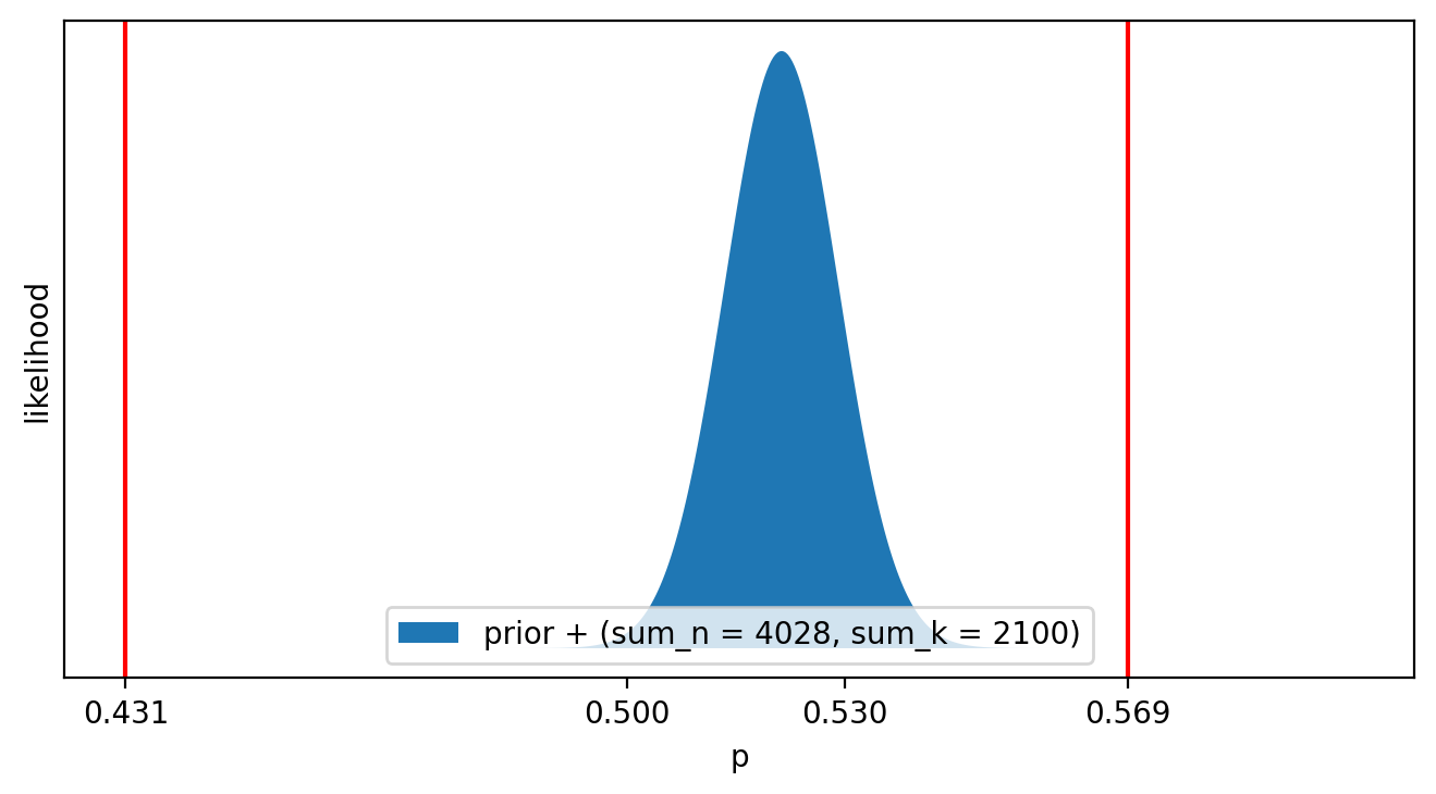
Fig. 4 The posterior when I target seven Blaze rods over the course of 300 runs, with a 53% chance of success.
The posterior appears to provide strong evidence that I altered my drop rate, as little credence is massed around \(p = \frac 1 2\). Yet almost all of the credence lies within the bounds of integration, so our calculated value is effectively identical to a perfectly fair Blaze rod drop rate.
The 56.9% definition of “fair enough” is for coin tosses, which are rarely done more than once or twice in a sitting. Blaze rod drops can be easily modelled by coin flips, and yet the above figure tells me I performed 4028 total flips. Our definition of “fair enough” depends on what we can detect, and the more events we observe the better we can detect subtle biases. It isn’t enough for \(H_\text{fair}\) to integrate over a range, its must “tighten up” as more data arrives.
Consider a version of Minecraft that swapped out the pseudo-random number generator with a sophisticated non-random algorithm. The game can detect the number of Blaze rods I want, and automatically ensure exactly half of the Blazes I kill will drop Blaze rods. If I fed this fair algorithm into the math and generated a posterior, for the \(\|\vec n\|_1 = 28\) case I would get
random  = np.random.default_rng(15)

k = 3     # number of Blaze rods needed
c = 5     # number of runs to earn k Blaze rods

sum_k = k * c  # we already know this
sum_n = 0

for experiment in range(c):
    results = random.choice( 2, size=16 )
    while np.sum(results) < k:
        results = np.append( results, random.choice( 2, size=16 ) )
    sum_n += np.sum( np.cumsum( results ) < k ) + 1

my_prior = prior(0.5, 4)

fig = plt.figure(figsize=(8, 4), dpi=dpi, facecolor='w', edgecolor='k')

x = np.linspace(0,1,512)
plt.fill_between( x, beta.pdf( x, my_prior[0] + sum_k, my_prior[1] + sum_n - sum_k), linestyle='-',
                label=f'prior + (sum_n = {sum_n}, sum_k = {sum_k})')

plt.plot( x, beta.pdf( x, my_prior[0] + sum_n/2, my_prior[1] + sum_n/2), '-k', \
         label=f'fair play (Beta({my_prior[0] + sum_n/2:.1f},{my_prior[1] + sum_n/2:.1f}))')
plt.axvline( 0.5, color='red' )

plt.xticks([0,.5,1])
plt.xlabel('p')

plt.yticks([])
plt.ylabel('likelihood')

plt.legend()
fig_show( fig, 'fig:fair_play' )
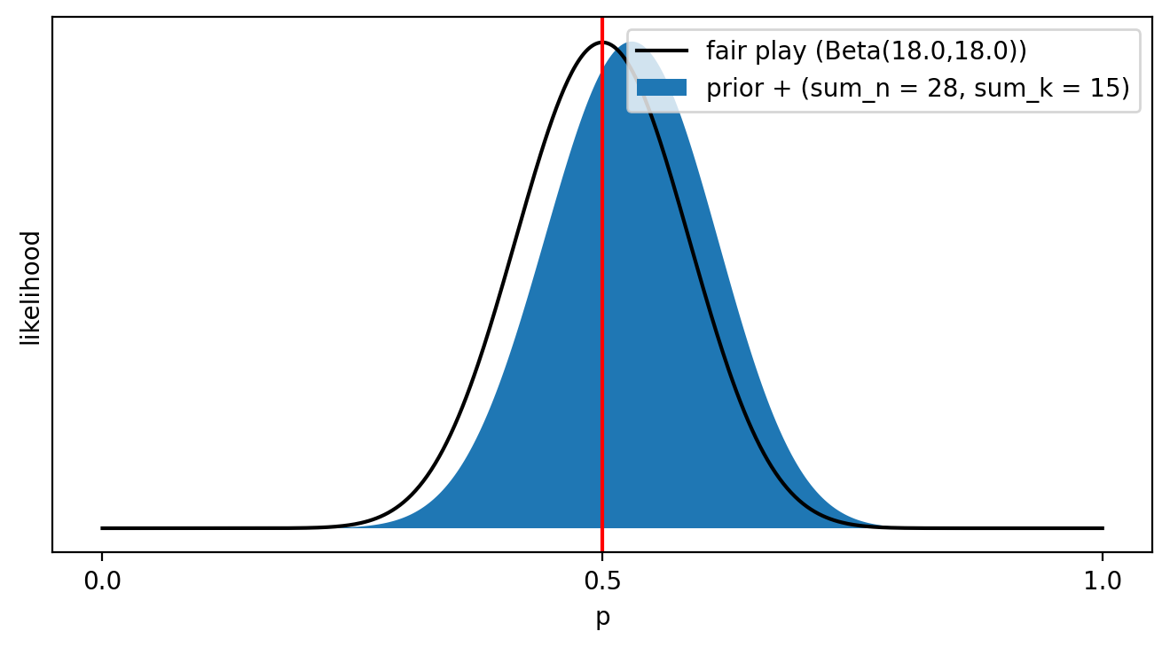
Fig. 5 The posterior after a perfectly fair play session, compared to the posterior for the last toy example of The Binomial and Negative Binomial Distributions.
I consider this posterior to be a really good match for \(H_\text{fair}\). You might have thought of a problem, though: what if I’d killed twenty-seven Blazes instead of twenty-eight? Or, for a more extreme example, a perfectly fair Ender pearl barter session is twenty successes for every 423 attempts. Those two numbers are co-prime, so the number of successful pearl barters will only be an integer if the number of attempts is a multiple of 423. It would be terribly inconvenient to force players to barter exactly 423 times so we can analyze their bartering rate.
Thankfully for us, the Gamma function is defined for fractions. For Ender pearl barters, we can construct \(H_\text{fair}\) by assigning \(\frac{20}{423}\) successes for every single barter, instead of twenty successes for every 423 barters. Now we can handle an arbitrary number of drops or barters.
Let’s lock the mathematics for \(H_\text{fair}(\|\vec n\|_1)\) down.
where \(r_\text{fair}\) is the rate we expect during fair play. For instace, \(r_\text{blaze} = \frac 1 2\) and \(r_\text{pearl} = \frac{20}{423}\).
If you do not agree with my definition of “fair play” according to Equation (20), I’d encourage you to think up your own and express it in a mathematically precise way. In the meantime, I’ll use my definition to create a likelihood from the posterior. To do that, I multiply \(H_\text{fair}(\|\vec n\|_1)\) by the Beta posterior and integrate the combination.
Equation (26) isn’t as tidy as we’d hoped, but at least that integral is gone. It looks very difficult to evaluate, but I have an ace up my sleeve. mpmath is a Python library that allows you to do calculations with arbitrary precision. This is handy when dealing with very large numbers, as conventional floating-point math breaks when the numbers get too big. One function in that library, mpmath.gammaprod(), allows you to calculate fractions with arbitrary numbers of Gamma functions in the numerator or denominator. It makes evaluating messes like Equation (26) a snap.
Let’s see it in action. I’ll fix \(\|\vec n\|_1\) = 28 and \(r_\text{fair} = \frac 1 2\), apply my prior of \(\alpha_\text{prior} = \beta_\text{prior} = 4\), and then enumerate all possible values of \(\|\vec k\|_1\) and plot them on a chart.
def posterior_H_fair( vec_k, vec_n, r_fair, a_prior, b_prior ):
    """Calculate the likelihood of H_fair, given the posterior distribution defined by vec_n, vec_k, and the prior.
        Relies on mpmath to perform all calculations, which also means you can adjust the precision.

    Parameters
    ----------
    vec_k: A total or list containing the successful attempts at this task until it was completed.
    vec_n: A total or list containing the total attempts at this task until it was completed.
    r_fair: A float between 0 and 1 representing the probability of success predicted by H_fair.
    a_prior: A positive or zero float representing the alpha variable of the prior.
    b_prior: A positive or zero float representing the beta variable of the prior.

    Returns
    -------
    The likelihood, an mpmath float in the range [0,infinity]."""

    # place some imports here to encourage copy-paste coding
    from mpmath import gammaprod
    from numpy import sum        # vectorized, likely faster than Python's sum

    # the downside of encouraging copy-pasting is that this code will face some
    #  dirty/invalid inputs. By going wild with asserts, I'm making it tougher to
    #  use this function inappropriately.
    assert (r_fair > 0) and (r_fair < 1)
    assert (a_prior >= 0) and (b_prior >= 0)

    # use duck typing to determine whether these are lists or not
    try:
        len_k = len(vec_k)
        k_is_list = True
    except TypeError:
        len_k = 1
        k_is_list = False

    try:
        len_n = len(vec_n)
        n_is_list = True
    except TypeError:
        len_n = 1
        n_is_list = False

    # do additional checks if both are lists
    if k_is_list and n_is_list:

        assert len_k == len_n
        for i,n in enumerate(vec_n):
            assert n > 0
            assert (vec_k[i] >= 0) and (vec_k[i] <= n)

    # now calculate sums
    if k_is_list:
        sum_k = sum(vec_k)
    else:
        sum_k = vec_k

    if n_is_list:
        sum_n = sum(vec_n)
    else:
        sum_n = vec_n

    # one final round of checks
    assert sum_n >= 1
    assert (sum_k >= 0) and (sum_k <= sum_n)

    # calculate the final result
    numerator =   [a_prior + b_prior + sum_n, a_prior + b_prior + sum_n,
                  2*a_prior + sum_k + r_fair*sum_n - 1,
                  2*b_prior - sum_k + (2 - r_fair)*sum_n - 1]
    denominator = [a_prior + sum_k, b_prior + sum_n - sum_k,
                   a_prior + r_fair*sum_n, b_prior + (1 -r_fair)*sum_n,
                  2*(a_prior + b_prior + sum_n - 1)]

    return gammaprod(numerator, denominator)
sum_n  = 28
glue( 'deffair_sum_n', sum_n, display=False )

r_fair = Fraction(1,2)
a_prior, b_prior = prior( r_fair, 4 )


fig = plt.figure(figsize=(8, 4), dpi=dpi, facecolor='w', edgecolor='k')

x = np.arange(sum_n + 1)
plt.bar( x, [posterior_H_fair( v, sum_n, r_fair, a_prior, b_prior ) for v in x], \
        label=f'sum_n = {sum_n}, prior = ({a_prior}, {b_prior})')

plt.ylabel("likelihood")
plt.yticks([ 0, 2, 3.5 ])

plt.xlabel('sum_k')
plt.xticks([ 0, sum_n >> 1, sum_n ])

plt.legend()
fig_show( fig, 'fig:posterior_H_fair' )
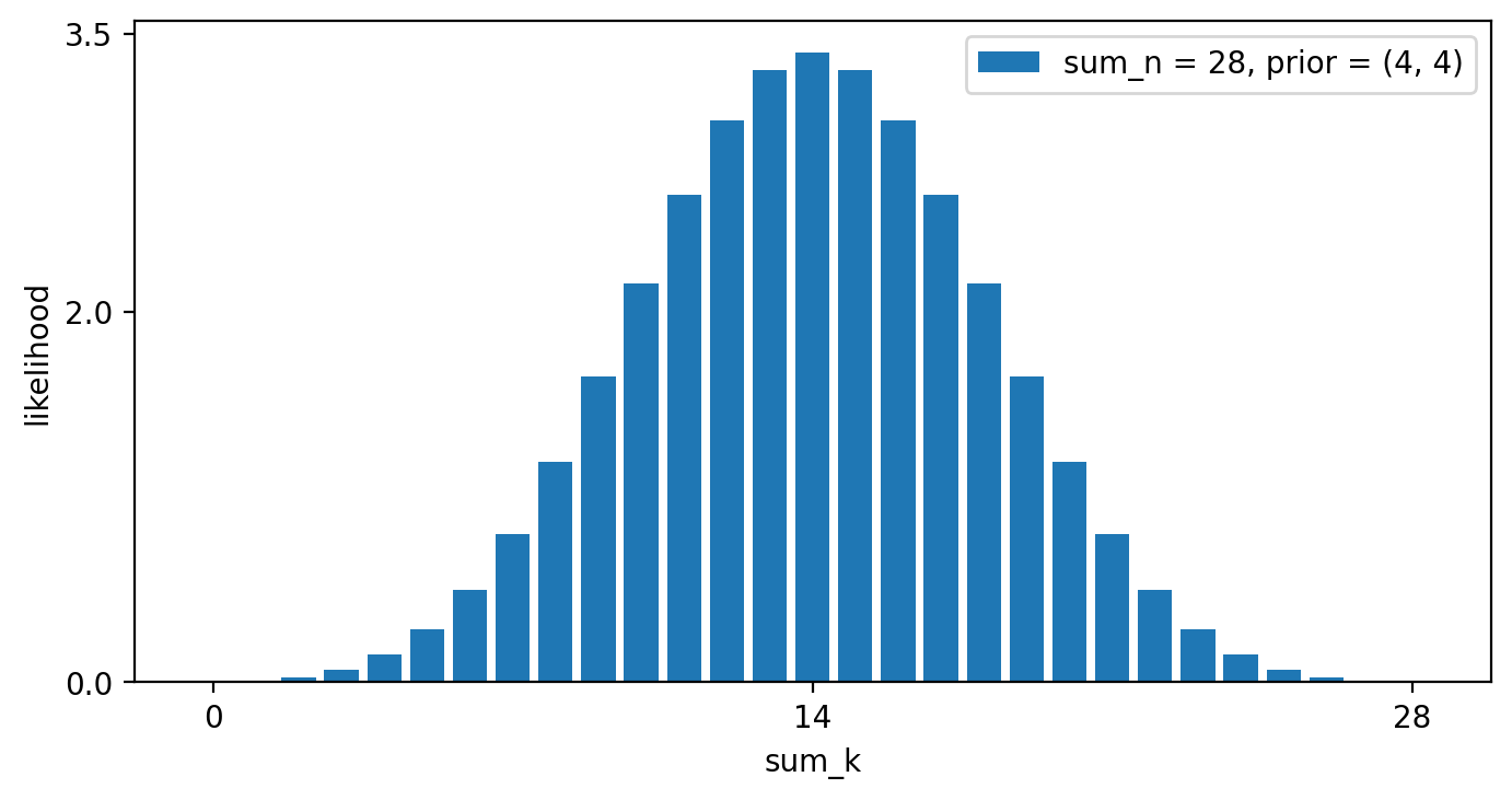
Fig. 6 The likelihood of all possible \(\|\vec k\|_1\) values, when \(\|\vec n\|_1\) = 28 and all other parameters are fixed.
This likelihood behaves much as we’d expect. \(H_\text{fair}(\|\vec n\|_1)\) is maximized when \(\|\vec k\|_1 = r_\text{fair}\|\vec n\|_1\), remains quite high for nearby values, but rapidly drops off as \(\|\vec k\|_1\) diverges.
Defining Cheating
We’re still dealing with raw likelihoods, though. As mentioned in Missing Context, we need a reference point. The usual solution is to calculate a Bayes factor.[KR95] You’ve likely seen Bayes’ Theorem,
The likelihood function \(p( E | H_1 )\) and prior \(p( H_1 )\) should be familiar. The normalization factor \(p( E )\) is the probability of observing the evidence over all possible hypotheses, and is the canonical reference point. “All possible” is not the same as “all,” so the most common way to evaluate it is to declare a handful of hypotheses as the only ones that are possible, evaluate their likelihoods, then calculate \(p(E) = p( E | H_1 )p(H_1) + p( E | H_2 )p(H_2) + \dots + p( E | H_j )p( H_j )\). Defining all those hypotheses can be difficult, and opens us up to charges of cooking the books.
An alternate approach is to define just one more hypothesis and divide.
Not only is \(p(E)\) eliminated, constants across the numerator and denominator cancel out. This “Bayes factor” has the same interpretation as betting odds, with numbers greater than 1 indicating \(H_1\) is favoured and vice-versa. It has none of the flaws of p-values. For instance, since it obeys all the properties of a likelihood you can combine multiple Bayes factors together by multiplying them, just as you do with probabilities.
In this context, the only worthwhile second hypothesis is “did Dream cheat?” Unfortunately, while there’s only one \(r_\text{fair}\) there are many ways to cheat. Ideally we’d consult with experts about Minecraft speedrunning and develop a mathematically-precise hypothesis about what cheating looks like. Since I do not have those connections, I’ll invoke a backup strat.
If we accept my definition of \(H_\text{fair}\), we can define \(H_\text{cheat}\) as the inverse of that definition; where \(H_\text{fair}\) asserts fair play is likely, \(H_\text{cheat}\) asserts it is unlikely, and vice-versa. The easiest way to accomplish that is to subtract the likelihood output by \(H_\text{fair}\) from some other value. This value must be high enough to prevent the result from ever being negative, and not so high that it waters down the hypothesis to look more like the Bayes/Laplace prior. The obvious choice is to use the maximal likelihood of \(H_\text{fair}\) as that value, which is
There are three flaws with using \(M_\text{fair} - H_\text{fair}\) as \(H_\text{cheat}\). This hypothesis gives maximal credence to both \(p = 0\) and \(p = 1\), and yet no cheater would dare set their probability of success to those values. Unfortunately, I can think of no non-trivial way to compensate for this.
This hypothesis also states that if \(\|\vec k\|_1 = r_\text{fair}\|\vec n\|_1\), the likelihood of cheating is zero. Yet we can easily concoct scenarios where a run of bad luck happens to result in a record that appears perfectly fair. In comparison, \(H_\text{fair}\) has no zeros except at \(p = 0\) and \(p = 1\). A better alternative is to add some small offset to model to capture the small but ever-present possibility of cheating. It would be wise to scale this offset by the inverse of \(\|\vec n\|_1\), to reflect the fact that as more data comes in we become more confident that cheating has not occurred.
I propose \(\frac 1 2 \|\vec n\|_1^{-1}\) is a good choice. Consider an ideal Bernoulli process representing evidence towards some hypothesis. As we know nothing about this process, “non-informative” priors make more sense than a subjective ones. I consider the best-justified “non-informative” prior to be Jeffreys’ prior, which in this case is \(\text{Beta}(\frac 1 2, \frac 1 2)\). If all \(\|\vec n\|_1\) atoms of evidence pulled from this process goes against the hypothesis, the mean value for the probability of truth \(p\) is
Naturally, there’s room for disagreement. If you think the Bayes/Laplace prior is less informative, then \(\|\vec n\|_1^{-1}\) is a better offset. I can keep the constant scalar separate, so if you prefer the Bayes/Laplace you can substitute 1 in for the Jeffreys \(\frac 1 2\), or even eliminate the offset entirely by setting the constant to zero.
Third and finally, \(M_\text{fair} - H_\text{fair} + \frac 1 2 \|\vec n\|_1^{-1}\) is not normalized when integrated by \(p\), a requirement if we’re to compare it against \(H_\text{fair}\). This is simple to fix, as
so therefore
and we can finally write out \(H_\text{cheat}\).
For the toy example above, Equation (33) looks like
random  = np.random.default_rng(15)

k = 3     # number of Blaze rods needed
c = 5     # number of runs to earn k Blaze rods

sum_k = k * c  # we already know this
sum_n = 0

for experiment in range(c):
    results = random.choice( 2, size=16 )
    while np.sum(results) < k:
        results = np.append( results, random.choice( 2, size=16 ) )
    sum_n += np.sum( np.cumsum( results ) < k ) + 1

my_prior = prior(0.5, 4)


fig = plt.figure(figsize=(8, 4), dpi=dpi, facecolor='w', edgecolor='k')

x = np.linspace(0,1,512)
m = (my_prior[0] + sum_n/2 - 1) / (sum(my_prior) + sum_n - 2)
M = beta.pdf( m, my_prior[0] + sum_n/2, my_prior[1] + sum_n/2)
plt.fill_between( x, (M - beta.pdf( x, my_prior[0] + sum_n/2, my_prior[1] + sum_n/2) + (.5/sum_n))/(M-1+(.5/sum_n)), \
         label=f'H_cheat (sum_n = {sum_n})')

plt.plot( x, beta.pdf( x, my_prior[0] + sum_n/2, my_prior[1] + sum_n/2), '-k', label=f'H_fair (sum_n = {sum_n})')
plt.axvline( 0.5, color='red' )


plt.xticks([0,.5,1])
plt.xlabel('p')

plt.yticks([0,1])
plt.ylabel('likelihood')

plt.legend()
fig_show( fig, 'fig:h_cheat_h_fair_toy' )
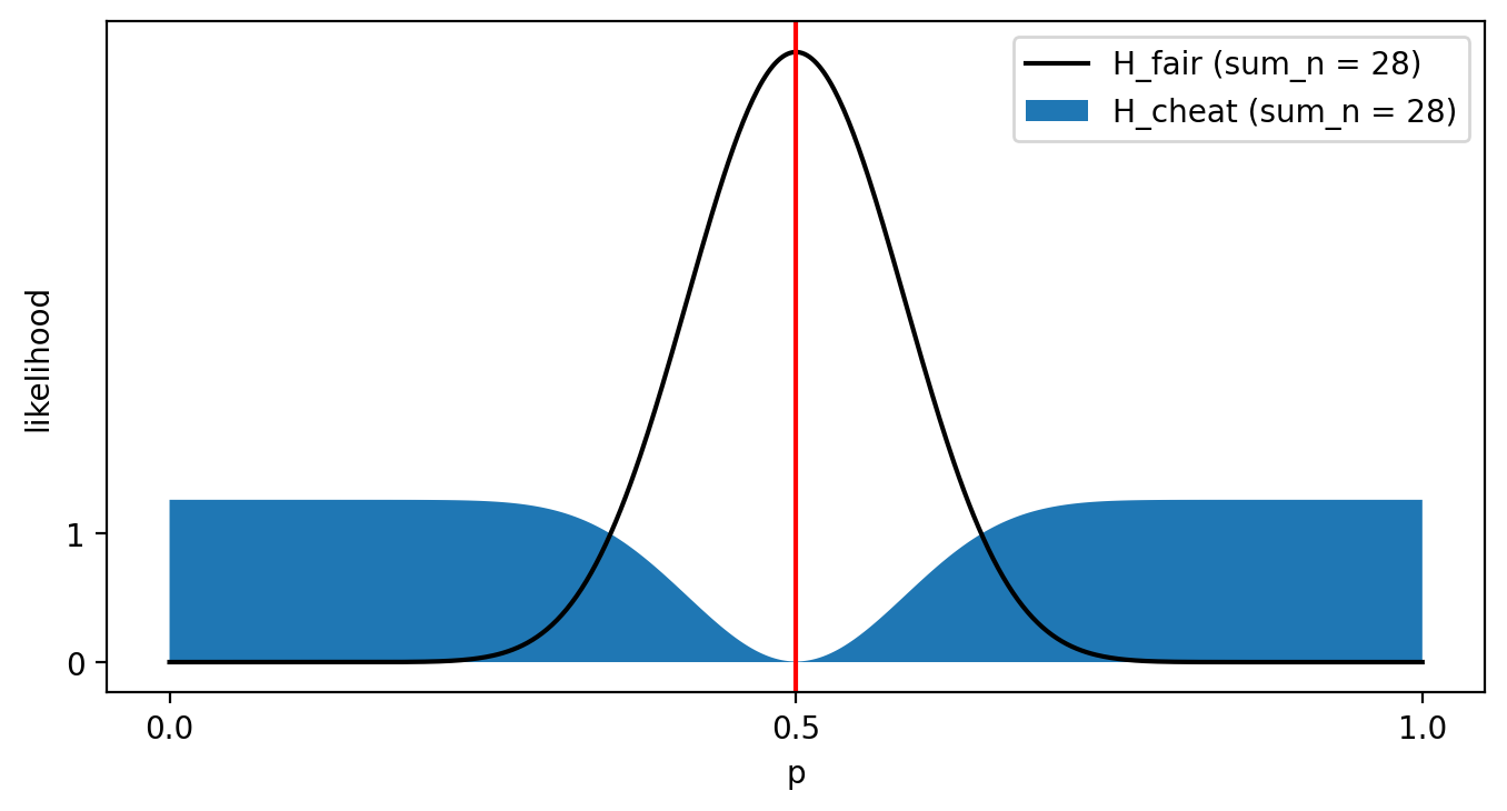
Fig. 7 Comparing \(H_\text{fair}\) with \(H_\text{cheat}\), applied to the toy example.
Putting It All Together
We finally have enough math in place to calculate a Bayes factor.
Notice that Equation (36) uses the same integral invoked to evaluate \(H_\text{fair}\) on the posterior, so I can recycle posterior_H_fair() to simplify the calculations.
def BF_H_fair_H_cheat( vec_k, vec_n, r_fair, a_prior, b_prior, sum_n_scalar=0.5 ):
    """Calculate the Bayes factor associated with H_fair / H_cheat, given the posterior distribution defined by vec_n, vec_k, and the prior.
        Relies on mpmath to perform all calculations, which also means you can adjust the precision.

    Parameters
    ----------
    vec_k: A total or list containing the successful attempts at this task until it was completed.
    vec_n: A total or list containing the total attempts at this task until it was completed.
    r_fair: A float between 0 and 1 representing the probability of success predicted by H_fair.
    a_prior: A positive or zero float representing the alpha variable of the prior.
    b_prior: A positive or zero float representing the beta variable of the prior.
    sum_n_scalar: A positive or zero float that's used to weight the ||vec_n|| component. Defaults to 1/2.

    Returns
    -------
    The Bayes factor, a likelihood and mpmath float in the range [0,infinity]. Values greater than 1 favour
       fairnes, values below 1 favour cheating."""

    from mpmath import fdiv, fmul, gammaprod, power

    # validate our one new variable
    assert sum_n_scalar >= 0

    # rely on posterior_H_fair()'s assertions to validate the remaining inputs
    integral = posterior_H_fair( vec_k, vec_n, r_fair, a_prior, b_prior )

    # but we still need sum_n for calculations
    try:
        len_n = len(vec_n)
        n_is_list = True
    except TypeError:
        len_n = 1
        n_is_list = False

    if n_is_list:
        sum_n = sum(vec_n)
    else:
        sum_n = vec_n


    # invoke mpmath instead of python's functions, to discourage precision loss
    m = fdiv( a_prior + r_fair*sum_n - 1,  a_prior + b_prior + sum_n - 2 )
    M = fmul( gammaprod([a_prior + b_prior + sum_n], [a_prior + r_fair*sum_n,b_prior + (1-r_fair)*sum_n]), \
             fmul(power( m, a_prior + r_fair*sum_n - 1 ), power( 1-m, b_prior + (1-r_fair)*sum_n - 1 )) )

    return fdiv( fmul(M - 1 + sum_n_scalar/sum_n, integral), M + sum_n_scalar/sum_n - integral )
Let’s see BF_H_fair_H_cheat() in action.
sum_n  = 28
r_fair = Fraction(1,2)
a_prior, b_prior = prior( r_fair, 4 )


fig = plt.figure(figsize=(8, 4), dpi=dpi, facecolor='w', edgecolor='k')

x = np.arange(sum_n + 1)
plt.plot( x, [BF_H_fair_H_cheat( v, sum_n, float(r_fair), a_prior, b_prior ) for v in x], '-', \
        label=f'sum_n = {sum_n}, prior = ({a_prior}, {b_prior})')
plt.plot( x, [1 for v in x], '-', \
        label='break even')

plt.ylabel("H_fair / H_cheat")
plt.yticks([0,1,2,4,8])

plt.xlabel('sum_k')
plt.xticks([ 0, 8, 14, 20, 28 ])

plt.legend()
fig_show( fig, 'fig:BF_posterior_H_fair' )
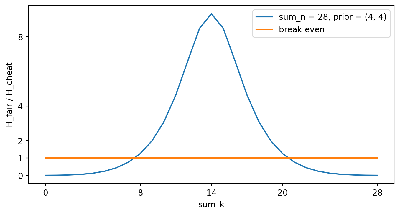
Fig. 8 The Bayes factor for all possible \(\|\vec k\|_1\) values, when \(\|\vec n\|_1\) = 28 and all other parameters are fixed.
The results are as expected. The sharper peak relative to the other chart with \(H_\text{fair}\) alone is due to the increasing likelihood of \(H_\text{cheat}\) given a \(\|\vec k\|_1\) that diverges from perfect fairness. Values of \(\|\vec k\|_1\) near \(r_\text{fair}\) are nonetheless considered net evidence in favour of \(H_\text{fair}\), while values far from there count as better evidence for \(H_\text{cheat}\). The crossover point is about six and a half possible values of \(\|\vec k\|_1\) away from perfect fairness in this case, though that point should be different for different \(\|\vec n\|_1\).
Another useful test is to fix \(\|\vec k\|_1 = \frac 1 2 \|\vec n\|_1\) and increase \(\|\vec n\|_1\). If you’ve done much frequentist analysis, you’ve noticed the term \(\sqrt{n}\) seems to pop up everywhere. This is a side-effect of the central limit theorem applied to “well-behaved” distributions, where it’s been proven that estimates of true mean will converge to that value at a rate proportional to \(\sqrt{n}\). We can think of that value as a metric for how strong the evidence is. Since Bernoulli processes are “well-behaved,” our evidence for any fixed hypothesis should show the same scaling factor.
r_fair = 0.5
a_prior, b_prior = prior( r_fair, 4 )


fig = plt.figure(figsize=(8, 4), dpi=dpi, facecolor='w', edgecolor='k')

x = np.exp( np.linspace(np.log(8), np.log(1 << 18), 256) )
plt.plot( x, [BF_H_fair_H_cheat( v/2, v, float(r_fair), a_prior, b_prior ) for v in x], '-', \
        label=f'maximal likelihood')

plt.plot( x, 1.9*np.sqrt(x), '-k', label='1.9 * sqrt(sum_n)' )

plt.ylabel("H_fair / H_cheat")
plt.yticks([1, 1000])

plt.xlabel('sum_n')
plt.xticks([8, 1 << 18])

plt.legend()
fig_show( fig, 'fig:weight_evidence' )
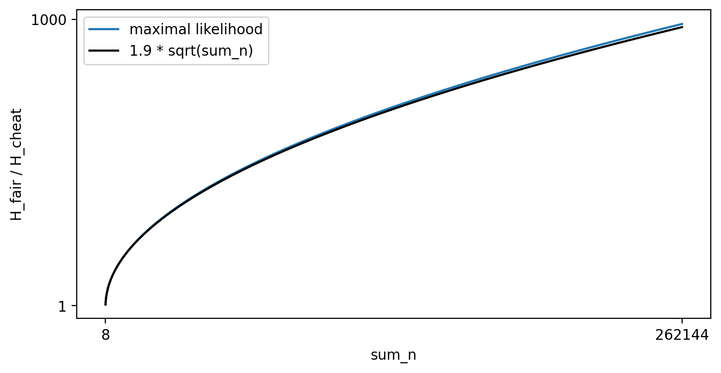
Fig. 9 How the Bayes factor increases when \(\|\vec k\|_1 = \frac 1 2 \|\vec n\|_1\).
Again, this chart holds no surprises, save a subtle divergence between the theoretical and practical behaviour of the Bayes factor. This is likely due to the \(\frac 1 2 \|\vec n\|_1^{-1}\) term adding some skew when \(\|\vec n\|_1\) is small.